Preprocessing and correcting sinograms

A Tutorial on sinogram handling

Overview

This tutorial introduces the key sinogram preprocessing functions in nDTomo, designed to handle raw pencil beam or 2D/3D parallel beam CT data before reconstruction. Preprocessing is essential to correct for experimental artefacts such as baseline offsets, beam intensity fluctuations, misalignment, and center of rotation drift — all of which can severely degrade the quality of the reconstructed image.

These tools operate on both 2D sinograms and 3D sinogram stacks (e.g., spectral or z-resolved data), and are modular so you can tailor your preprocessing pipeline to your specific dataset and experimental setup.

Objectives

By the end of this tutorial, you will:

• Apply nDTomo functions to correct background offsets, beam drift, motor jitter, and rotation misalignment.

• Understand how each function transforms the sinogram and why it’s necessary.

• Build a robust preprocessing workflow for high-quality tomographic reconstruction.

Sinogram Preprocessing Functions

1. ``airrem`` – Air Background Removal

Removes additive background signal (air signal) by estimating and subtracting it from edge rows of the sinogram. This is useful when portions of the sinogram (top/bottom) contain no sample.

• Modes: "both", "top", "bottom" — determines where to sample air signal

• Offset (``ofs``): Number of rows used to estimate the background

• Column selection (``coli``, ``colf``): Restrict estimation to specific columns

• Supports: 2D and 3D sinograms (correction applied per projection)

Why use it?

To suppress air-related background levels that would otherwise interfere with reconstruction or downstream fitting.

2. ``scalesinos`` – Sinogram Normalization

Normalizes each projection by its total integrated intensity to account for fluctuations in beam intensity or sample attenuation.

• Computes a scaling factor per projection

• Divides each projection to normalize its sum relative to the maximum

• Automatically handles 2D and 3D sinograms

Why use it?

To equalize projection contributions and reduce artefacts from flux instability, detector gain drift, or sample thickness variations.

3. ``sinocentering`` – Center of Rotation (COR) Alignment

Identifies and corrects the center of rotation offset by comparing projections at 0° and 180°.

• Searches for COR by minimizing the standard deviation of flipped projections

• Works with 180° or 360° scans

• Optionally selects spectral channels to use

• Applies correction using interpolation

• Supports 2D and 3D inputs

Why use it?

To ensure the reconstructed image is centered and symmetric. Misaligned rotation axes produce severe artefacts and incorrect geometries.

4. ``sinocomcor`` – Common-Mode Correction / Motor Jitter Correction

Aligns projections based on their center of mass (COM), compensating for scan motor jitter or random translation shifts.

• Uses the COM of each projection

• Shifts projections using linear interpolation

• Works for 2D and 3D sinograms

Why use it?

To correct for lateral misalignments between projections caused by motor jitter or detector drift, improving reconstruction sharpness.

How This Tutorial Works

• We begin with a raw sinogram or stack of sinograms.

• Each preprocessing step is visualized to show its effect.

• Intermediate results are plotted after each correction.

• The final output is a clean, centered, and normalized sinogram ready for reconstruction (e.g., via filtered backprojection or DLSR).

Why This Matters

• Preprocessing directly impacts the fidelity of tomographic reconstructions

• Many artefacts (e.g., ringing, misalignments, loss of contrast) can be traced back to poor sinogram conditioning

• These tools provide a physically informed, user-adjustable, and lightweight preprocessing pipeline for pencil beam CT

Let’s now apply each of these functions in sequence and observe their effects.

import numpy as np
import matplotlib.pyplot as plt
from skimage.transform import iradon, radon
from tqdm import tqdm

from nDTomo.sim.phantoms import SheppLogan
from nDTomo.methods.xrays import simulate_synchrotron_intensity
from nDTomo.tomo.sinograms import scalesinos, airrem, sinocomcor, sinocentering

WARNING:silx.opencl.common:Unable to import pyOpenCl. Please install it from: https://pypi.org/project/pyopencl

First we create a phantom object that we will use for our simulations

npix = 128
img = SheppLogan(npix)

plt.figure(1);plt.clf()
plt.imshow(img, cmap='gray')
plt.title('Shepp-Logan Phantom')
plt.colorbar()
plt.show()

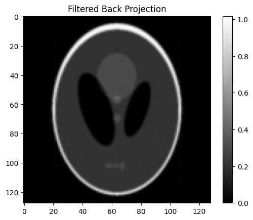
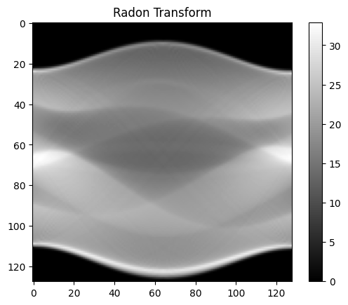
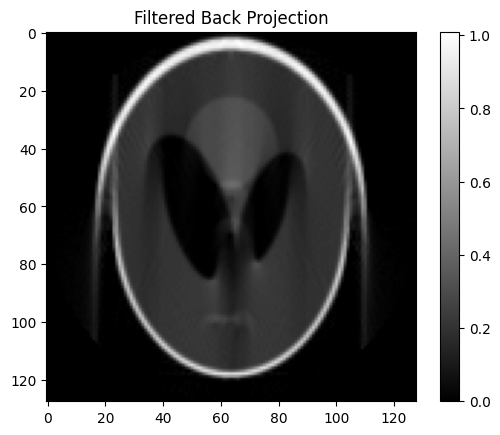
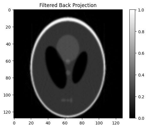
Initial FBP Reconstruction Without Artefacts

Before applying any corrections or artefact removal steps, it’s important to visualize the baseline performance of filtered back projection (FBP) on a clean synthetic sinogram. This provides a reference for evaluating the impact of subsequent preprocessing steps.

In this section, we perform FBP reconstruction on a simulated sinogram (e.g., Shepp-Logan phantom) without introducing any noise, background signal, or alignment issues. This allows us to confirm that:

• The sinogram is correctly generated.

• The FBP algorithm is functioning as expected.

• The spatial resolution and feature contrast are consistent with the known phantom structure.

This reconstruction serves as a “ground truth” benchmark, and visual comparison with corrected versions later helps quantify improvements.

scan = 180
theta = np.arange(0, scan, scan/npix)
print('The number of angles is', len(theta))

s = radon(img, theta)

fbp = iradon(s, theta, filter_name='ramp', output_size=npix)
fbp[fbp < 0] = 0

plt.figure(1);plt.clf()
plt.imshow(s, cmap='gray')
plt.title('Radon Transform')
plt.colorbar()
plt.show()

plt.figure(2);plt.clf()
plt.imshow(fbp, cmap='gray')
plt.title('Filtered Back Projection')
plt.colorbar()
plt.show()

The number of angles is 128

Air Signal Removal from Sinograms

During X-ray CT sinograms often include a background signal from air attenuation or scattering that does not contain useful sample information. This background appears as a constant or slowly varying offset in each projection.

The airrem function removes this unwanted background signal by averaging pixel intensities at the edges of the sinogram—either the top, bottom, or both—and subtracting this average from the entire projection.

Key benefits of this step:

• Enhances image contrast in reconstructions.

• Reduces artefacts caused by detector offsets or flat-field mismatch.

• Makes subsequent corrections (e.g., centering, alignment) more robust.

You can tune how many rows are used (ofs) and restrict the averaging to a subset of columns (coli, colf) if needed.

sn = np.copy(s)

bkg = 20
sn = sn + bkg

fbp = iradon(sn, theta, filter_name='ramp', output_size=npix)
fbp[fbp < 0] = 0

plt.figure(1);plt.clf()
plt.imshow(sn, cmap='gray')
plt.title('Radon Transform')
plt.colorbar()
plt.show()

plt.figure(2);plt.clf()
plt.imshow(fbp, cmap='gray')
plt.title('Filtered Back Projection')
plt.colorbar()
plt.show()


sn = airrem(sn, ofs = 2, method="both", coli=0, colf=2)
fbp = iradon(sn, theta, filter_name='ramp', output_size=npix)
fbp[fbp < 0] = 0

plt.figure(1);plt.clf()
plt.imshow(sn, cmap='gray')
plt.title('Radon Transform')
plt.colorbar()
plt.show()

plt.figure(2);plt.clf()
plt.imshow(fbp, cmap='gray')
plt.title('Filtered Back Projection')
plt.colorbar()
plt.show()

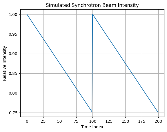
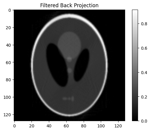
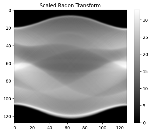
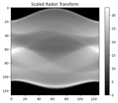
Sinogram Normalization Using scalesinos

In many tomographic experiments, it’s assumed that the total X-ray intensity (i.e., total scattering or transmission) for each projection should remain constant. However, experimental conditions such as beam fluctuations, sample movement, or detector drift can introduce global intensity variations across projections.

The scalesinos function corrects for these variations by normalizing each projection based on its total integrated intensity. Specifically, it computes the sum of all pixel values in each projection, compares this to the maximum total intensity observed, and scales the projection accordingly.

This normalization ensures that:

• Each projection contributes equally to the final reconstruction.

• Global contrast fluctuations are minimized.

• Reconstructions are more robust to beam instabilities and sample positioning errors.

For 3D sinograms, the normalization is applied slice-by-slice across the spectral or z-dimension.

To demonstrate this, we introduce artificial beam fluctuations using the simulate_synchrotron_intensity function. This generates a 1D intensity profile that mimics periodic decay and top-up cycles at a synchrotron source. By multiplying each projection by this synthetic profile, we simulate the effect of non-uniform beam exposure, which scalesinos is then used to correct.

sf = simulate_synchrotron_intensity(200, 0.75, num_topups=2)

plt.figure(1);plt.clf()
plt.plot(sf)
plt.title("Simulated Synchrotron Beam Intensity")
plt.xlabel("Time Index")
plt.ylabel("Relative Intensity")
plt.grid(True)
plt.show()

sn = np.copy(s)

for ii in range(sn.shape[1]):
    sn[:, ii] = sn[:, ii] * sf[ii]

fbp = iradon(sn, theta, filter_name='ramp', output_size=npix)
fbp[fbp < 0] = 0

plt.figure(1);plt.clf()
plt.imshow(sn, cmap='gray')
plt.title('Radon Transform')
plt.colorbar()
plt.show()

plt.figure(2);plt.clf()
plt.imshow(fbp, cmap='gray')
plt.title('Filtered Back Projection')
plt.colorbar()
plt.show()

sn = scalesinos(sn)
fbp = iradon(sn, theta, filter_name='ramp', output_size=npix)
fbp[fbp < 0] = 0

plt.figure(1);plt.clf()
plt.imshow(sn, cmap='gray')
plt.title('Scaled Radon Transform')
plt.colorbar()
plt.show()

plt.figure(2);plt.clf()
plt.imshow(fbp, cmap='gray')
plt.title('Filtered Back Projection')
plt.colorbar()
plt.show()

Rotation Axis Correction Using sinocentering

Precise knowledge of the center of rotation (COR) is essential for accurate tomographic reconstruction. If the COR is misaligned, it can introduce severe artefacts such as doubling, blurring, or streaking in the reconstructed image.

The sinocentering function estimates and applies a correction for COR misalignment by:

1. Comparing the projection at 0° with the flipped projection at 180°.

2. Searching within a user-defined range (crsr) for the optimal COR that minimizes the standard deviation between the two.

3. Shifting the sinogram data accordingly using linear interpolation.

Key features of sinocentering:

• Supports both 2D and 3D sinograms.

• The correction is applied uniformly across the entire sinogram or volume.

• In 3D mode, a subset of spectral channels can be specified via the channels parameter. These selected channels are used only for computing the COR — the correction is then applied to all channels uniformly. This is useful when some channels contain artefacts or noise that could bias the COR estimation.

• Handles both 180° and 360° scans using the scan parameter.

• Provides an optional progress bar during execution (pbar=True).

This function is typically used after motor jitter correction (sinocomcor) and intensity normalization, and just before reconstruction.

sn = np.copy(s)

ofs = 3
sn = np.roll(sn, ofs, axis = 0)

fbp = iradon(sn, theta, filter_name='ramp', output_size=npix)
fbp[fbp < 0] = 0

plt.figure(1);plt.clf()
plt.imshow(sn, cmap='gray')
plt.title('Radon Transform')
plt.colorbar()
plt.show()

plt.figure(2);plt.clf()
plt.imshow(fbp, cmap='gray')
plt.title('Filtered Back Projection')
plt.colorbar()
plt.show()

sn = sinocentering(sn, crsr=5, interp=True, scan=180, channels = None, pbar=True)
fbp = iradon(sn, theta, filter_name='ramp', output_size=npix)
fbp[fbp < 0] = 0

plt.figure(1);plt.clf()
plt.imshow(sn, cmap='gray')
plt.title('Radon Transform')
plt.colorbar()
plt.show()

plt.figure(2);plt.clf()
plt.imshow(fbp, cmap='gray')
plt.title('Filtered Back Projection')
plt.colorbar()
plt.show()

Calculating the COR

100%|██████████| 100/100 [00:00<00:00, 898.41it/s]

Calculated COR: 68.00000000000013
Applying the COR correction

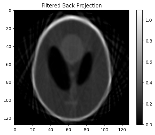
Motor Jitter Correction Using Center of Mass (COM) Alignment

Mechanical instabilities or motor jitter can cause each projection in a sinogram to be slightly misaligned along the translation axis. These small shifts accumulate and lead to blurred or distorted reconstructions.

The sinocomcor function corrects these shifts by:

1. Computing the center of mass (COM) for each projection using its intensity profile.

2. Aligning all projections so that their COM matches that of the first projection.

3. Applying this correction using linear interpolation, optionally clipping extrapolated values.

This correction improves:

• Edge sharpness and alignment in reconstructions.

• The quality of subsequent centering or segmentation steps.

• Accuracy in time-resolved or dynamic tomography.

By default, the COM correction uses raw offsets, but more advanced options are also available.

sn = np.copy(s)

for ii in range(1, sn.shape[1]):
    ofs = np.random.randint(-3, 3)
    sn[:, ii] = np.roll(sn[:, ii], ofs)


fbp = iradon(sn, theta, filter_name='ramp', output_size=npix)
fbp[fbp < 0] = 0

plt.figure(1);plt.clf()
plt.imshow(sn, cmap='gray')
plt.title('Radon Transform')
plt.colorbar()
plt.show()

plt.figure(2);plt.clf()
plt.imshow(fbp, cmap='gray')
plt.title('Filtered Back Projection')
plt.colorbar()
plt.show()

sn = sinocomcor(sn, interp=False)
sn = sinocentering(sn, crsr=5, interp=True, scan=180, channels = None, pbar=False)

fbp = iradon(sn, theta, filter_name='ramp', output_size=npix)
fbp[fbp < 0] = 0

plt.figure(1);plt.clf()
plt.imshow(sn, cmap='gray')
plt.title('Scaled Radon Transform')
plt.colorbar()
plt.show()


plt.figure(2);plt.clf()
plt.imshow(fbp, cmap='gray')
plt.title('Filtered Back Projection')
plt.colorbar()
plt.show()

Sine Wave-Based COM Correction for Periodic Jitter

In some imaging setups, misalignments caused by mechanical vibrations may follow a periodic pattern, such as sinusoidal drift from oscillating components or rotating stages.

The sinocomcor function provides an option (sine_wave=True) to fit a sine wave to the computed COM offsets. This fitted curve is then used to correct the projections, rather than using noisy raw COM data.

Advantages of sine fitting:

• Provides smoother and more physically realistic corrections.

• Reduces sensitivity to noise in individual projections.

• Captures periodic trends in the system’s mechanical behavior.

If sine_wave_plot=True is enabled, the function will also generate a diagnostic plot showing the raw COM offsets and the fitted sine curve. This helps verify that the fit is appropriate and aligns with the observed misalignment pattern.

Use this option when you suspect the jitter is not random but instead driven by periodic motion.

sn = np.copy(s)

xold = np.arange(sn.shape[0])
for ii in range(1, sn.shape[1]):
    ofs = np.random.rand(1)[0]*3
    xnew = xold + ofs
    sn[:, ii] = np.interp(xnew, xold, sn[:, ii], left=0, right=0)

fbp = iradon(sn, theta, filter_name='ramp', output_size=npix)
fbp[fbp < 0] = 0

plt.figure(1);plt.clf()
plt.imshow(sn, cmap='gray')
plt.title('Radon Transform')
plt.colorbar()
plt.show()

plt.figure(2);plt.clf()
plt.imshow(fbp, cmap='gray')
plt.title('Filtered Back Projection')
plt.colorbar()
plt.show()

sn = sinocomcor(sn, interp=False, sine_wave=True, sine_wave_plot=True, pbar = False)
sn = sinocentering(sn, crsr=5, interp=True, scan=180, channels = None, pbar=True)

plt.figure(1);plt.clf()
plt.imshow(sn, cmap='gray')
plt.title('Radon Transform')
plt.colorbar()
plt.show()

fbp = iradon(sn, theta, filter_name='ramp', output_size=npix)
fbp[fbp < 0] = 0

plt.figure(2);plt.clf()
plt.imshow(fbp, cmap='gray')
plt.title('Filtered Back Projection')
plt.colorbar()
plt.show()

Calculating the COR

100%|██████████| 100/100 [00:00<00:00, 1315.73it/s]

Calculated COR: 63.70000000000007
Applying the COR correction

✅ Summary and Best Practices for Sinogram Preprocessing

In this tutorial, we demonstrated how to preprocess sinograms using nDTomo’s dedicated correction functions. These operations are essential for cleaning raw tomography data and ensuring accurate reconstructions.

🧰 Key Functions Used:

• airrem: Removed air/background signal using edge rows.

• scalesinos: Normalized projections to compensate for beam fluctuations.

• sinocentering: Estimated and corrected the center of rotation offset.

• sinocomcor: Aligned projections by their center of mass to correct for motor jitter.

• sinocomcor (sine_wave=True): Applied a smoothed periodic correction for systematic oscillations.

Each of these steps contributes to improving image quality by removing different classes of artefacts that commonly arise in experimental setups.

🔬 Why This Matters:

Preprocessing directly affects the fidelity of reconstructions. Correcting for intensity fluctuations, misalignments, and air signal ensures that downstream steps — whether filtered backprojection, iterative reconstruction, or spectral fitting — yield interpretable and reliable results.

🚀 Next Steps:

• Apply the full preprocessing pipeline to your own experimental sinograms.

• Explore the impact of each correction on real data using Napari or your preferred visualisation tool.

Well-preprocessed sinograms are the foundation of high-quality tomographic imaging.