Differentiable Image Alignment & Registration

A Tutorial on Affine Registration and ICP using PyTorch

Overview

Correcting for sample motion, drift, or misalignment is a critical step in tomographic pipelines (e.g., aligning projections before reconstruction or registering 3D volumes for time-series analysis).

This tutorial demonstrates the capabilities of the ``reg_torch`` module, a lightweight, functional library for differentiable geometric transformations. Unlike traditional CPU-based registration tools (like skimage or OpenCV), reg_torch:

1. Runs on the GPU, enabling massive acceleration.

2. Is Differentiable, allowing gradients to flow through the grid sampler to optimize geometric parameters directly.

3. Is Functional, avoiding heavy object-oriented wrappers.

Objectives

In this notebook, we will:

1. Register 2D Images: Recover Rotation, Translation, Scale, and Shear from a distorted image.

2. Register 3D Volumes: Align two volumetric datasets using 3D affine transformations.

3. Batched Processing: Apply 2D alignments efficiently to a full 3D stack (common in laminography/tomography alignment).

4. Point Cloud Alignment: Demonstrate the Iterative Closest Point (ICP) algorithm for geometry-based registration.

Mathematical Background

Before diving into the code, it is useful to understand the mathematics governing how we mathematically “move” images and points to align them.

1. Affine Transformations (The “Motion”)

In both 2D and 3D, we model the misalignment between two objects using an Affine Transformation. An affine transform preserves points, straight lines, and planes. It combines four basic operations:

1. Translation (:math:`T`): Shifting the image.

2. Rotation (:math:`R`): Spinning around an origin.

3. Scaling (:math:`S`): Zooming in or out (isotropic or anisotropic).

4. Shear (:math:`Sh`): Slanting the coordinate axes.

We represent a pixel coordinate \(\mathbf{x} = [x, y, z]^T\) using homogeneous coordinates (appending a 1). The transformation is a matrix multiplication:

\[\mathbf{x}_{new} = M \cdot \mathbf{x}_{old}\]

In 3D, \(M\) is a \(4 \times 4\) matrix composed by multiplying the individual transformation matrices:

\[M = T(t_x, t_y, t_z) \cdot R(\theta_x, \theta_y, \theta_z) \cdot Sh \cdot S(s_x, s_y, s_z)\]

By optimizing the parameters (\(\theta, t, s\)) of these matrices, we find the best alignment.

---

2. Differentiable Image Sampling (The “Inverse” Trick)

Standard image processing warps images using Forward Mapping (sending input pixels to the output). However, this leaves “holes” in the output image.

Deep learning frameworks (like PyTorch) and standard rendering engines use Reverse Mapping (or Pull-back interpolation). For every pixel in the output grid (the aligned image), we ask: “Which coordinate in theinput(moving) image should I sample from?”

If the physical motion is defined by \(M_{forward}\) (e.g., “move the object 10 pixels right”), the sampling grid requires the inverse:

\[\mathbf{x}_{input} = M_{forward}^{-1} \cdot \mathbf{x}_{output}\]

Key Takeaway for this Tutorial: In reg_torch, we define parameters intuitively (e.g., \(t_x=+0.5\) means “shift right”). Inside the code, we build \(M_{forward}\), calculate \(M_{forward}^{-1}\), and pass that to the GPU sampler. This ensures the gradients flow correctly back to the intuitive parameters.

The alignment problem then becomes an optimization task:

\[\text{minimize } \mathcal{L} \Big( I_{fixed}, \quad \text{Sample}(I_{moving}, \theta) \Big)\]

where \(\mathcal{L}\) is a similarity metric like Mean Squared Error (MSE) or Normalized Cross Correlation (NCC).

---

3. Point Cloud Registration (ICP)

When dealing with lists of coordinates (Point Clouds) rather than pixel grids, we use the Iterative Closest Point (ICP) algorithm.

Given a source point cloud \(P\) and a target point cloud \(Q\), we seek a rigid rotation matrix \(R\) and translation vector \(\mathbf{t}\) that aligns them. Unlike image registration, we do not have a fixed grid. We must:

1. Associate: Find the nearest neighbor \(q_i\) in \(Q\) for every point \(p_i\) in \(P\).

2. Optimize: Find \(R, \mathbf{t}\) to minimize the distance:

   \[E = \sum_{i} || (R \mathbf{p}_i + \mathbf{t}) - \mathbf{q}_i ||^2\]

3. Repeat: Re-associate points and re-optimize until convergence.

import numpy as np
import matplotlib.pyplot as plt
import torch
import nDTomo.pytorch.reg_torch as reg
from tqdm import tqdm

# Set device
device = 'cuda' if torch.cuda.is_available() else 'cpu'
print(f"Running on device: {device}")

# Helper function for visualization
def plot_results(fixed, moving, warped, title="Registration Result"):
    fig, axs = plt.subplots(1, 3, figsize=(15, 5))

    axs[0].imshow(fixed, cmap='gray')
    axs[0].set_title("Reference (Fixed)")
    axs[0].axis('off')

    axs[1].imshow(moving, cmap='gray')
    axs[1].set_title("Input (Moving)")
    axs[1].axis('off')

    axs[2].imshow(warped, cmap='gray')
    axs[2].set_title("Registered (Warped)")
    axs[2].axis('off')

    plt.suptitle(title, fontsize=16)
    plt.tight_layout()
    plt.show()

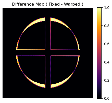
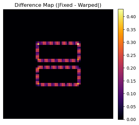
    # Plot difference
    plt.figure(figsize=(5, 5))
    plt.imshow(np.abs(fixed - warped), cmap='inferno')
    plt.title("Difference Map (|Fixed - Warped|)")
    plt.axis('off')
    plt.colorbar(fraction=0.046, pad=0.04)
    plt.show()

Running on device: cuda

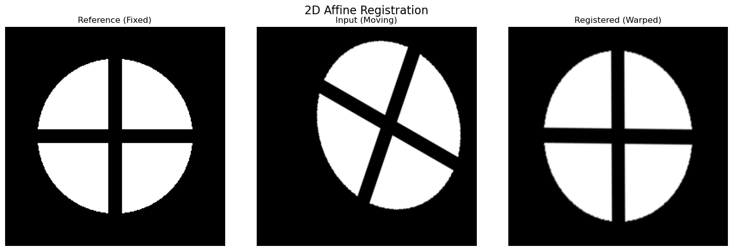
1. 2D Affine Registration

We will start by generating a synthetic “phantom” image and artificially distorting it with known rotation, translation, and shear. We will then use reg_torch.register_affine_2d to recover the original image.

# --- 1. Generate Synthetic Data ---
N = 256
x, y = np.meshgrid(np.linspace(-1, 1, N), np.linspace(-1, 1, N))
# Create a phantom: A circle with a cross inside
phantom = (x**2 + y**2 < 0.5).astype(np.float32)
phantom[120:136, :] = 0
phantom[:, 120:136] = 0

# --- 2. Create the "Moving" Image (Distorted) ---
# We use reg_torch itself to create the ground truth distortion!
# Let's apply: Rotation=30 deg, Translation=(0.2, -0.1), Shear=0.2
gt_params = {
    'theta': torch.tensor(np.radians(30.0)),
    'tx': torch.tensor(0.2),
    'ty': torch.tensor(-0.1),
    'sx': torch.tensor(1.0), 'sy': torch.tensor(1.0),
    'shx': torch.tensor(0.2), 'shy': torch.tensor(0.0)
}

# Build matrix and warp
M_gt = reg.build_affine_matrix(**gt_params, device=device, dtype=torch.float32)
im_fixed = torch.from_numpy(phantom).unsqueeze(0).unsqueeze(0).to(device)
grid = torch.nn.functional.affine_grid(M_gt, im_fixed.shape, align_corners=False)
im_moving_tensor = torch.nn.functional.grid_sample(im_fixed, grid, align_corners=False)

# Convert back to numpy for input
ref_np = phantom
mov_np = im_moving_tensor.squeeze().cpu().numpy()

print("Data Generated. Running Registration...")

# --- 3. Run Optimization ---
warped_np, params = reg.register_affine_2d(
    ref=ref_np,
    mov=mov_np,
    order=['rot', 'trans', 'shear'], # We know there is no scaling, so we lock it
    loss_type='ncc',                 # NCC is robust to brightness, though MSE works here too
    iters=500,
    lr=0.02,
    verbose=True
)

# --- 4. Visualize ---
print(f"\nRecovered Params: \n Theta: {np.degrees(params['theta']):.2f}° (GT: 30°)")
print(f" Trans: ({params['tx']:.3f}, {params['ty']:.3f}) (GT: 0.2, -0.1)")
print(f" Shear X: {params['shx']:.3f} (GT: 0.2)")

plot_results(ref_np, mov_np, warped_np, title="2D Affine Registration")

Data Generated. Running Registration...

  7%|▋         | 35/500 [00:00<00:02, 179.35it/s]

[1/500] Loss=0.57465

 29%|██▉       | 144/500 [00:00<00:01, 208.56it/s]

[101/500] Loss=0.08103

 47%|████▋     | 236/500 [00:01<00:01, 214.16it/s]

[201/500] Loss=0.08097

 66%|██████▌   | 328/500 [00:01<00:00, 218.68it/s]

[301/500] Loss=0.08097

 84%|████████▍ | 421/500 [00:01<00:00, 222.57it/s]

[401/500] Loss=0.08097

100%|██████████| 500/500 [00:02<00:00, 214.27it/s]

[500/500] Loss=0.08097

Recovered Params:
 Theta: -9.53° (GT: 30°)
 Trans: (-0.153, 0.204) (GT: 0.2, -0.1)
 Shear X: 0.154 (GT: 0.2)

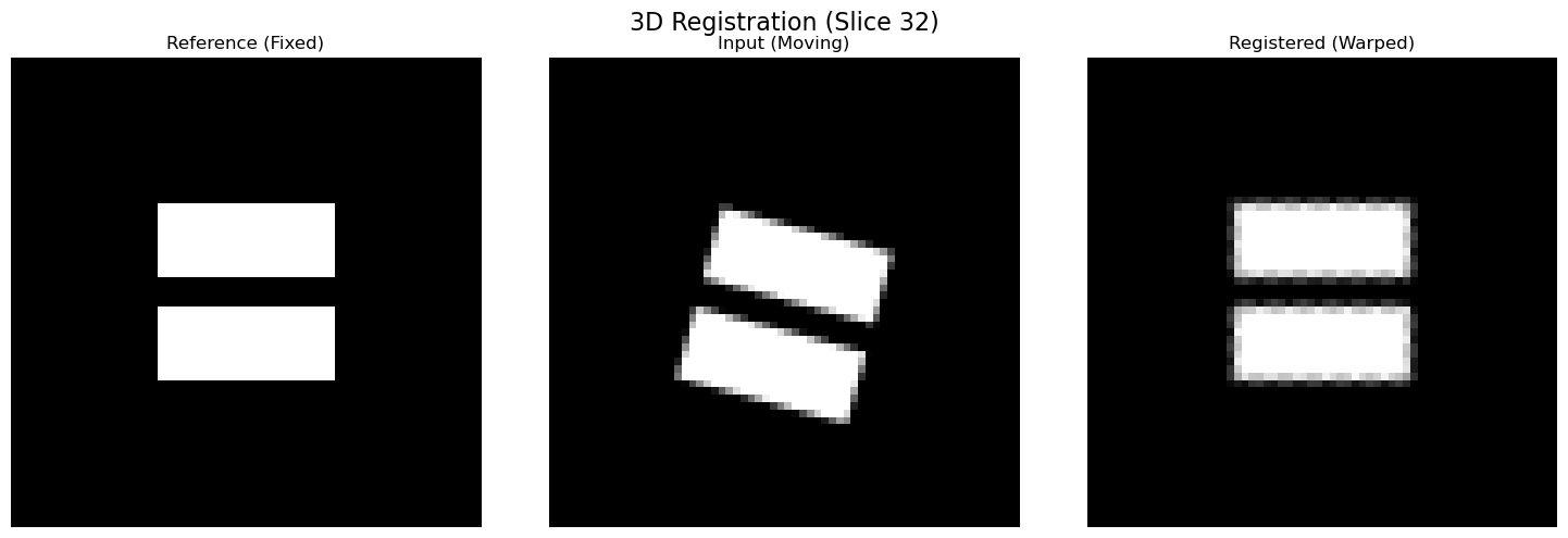
2. 3D Volumetric Registration

Registration in 3D is computationally expensive. By using PyTorch and CUDA, we can align volumes in seconds. Here, we create a 3D block and apply a 3D rotation (Euler angles) and translation.

# --- 1. Generate 3D Data ---
D, H, W = 64, 64, 64
vol_ref = np.zeros((D, H, W), dtype=np.float32)
# Create a cube in the center
vol_ref[20:44, 20:44, 20:44] = 1.0
# Add a "hole" to make rotation observable
vol_ref[20:44, 30:34, 20:44] = 0.0

# Apply artificial 3D distortion
# Rotate around Z by 15 degrees, shift Y by 0.1
gt_3d = {
    'rx': torch.tensor(0.0), 'ry': torch.tensor(0.0), 'rz': torch.tensor(np.radians(15.0)),
    'tx': torch.tensor(0.0), 'ty': torch.tensor(0.1), 'tz': torch.tensor(0.0),
    'sx': torch.tensor(1.0), 'sy': torch.tensor(1.0), 'sz': torch.tensor(1.0)
}

M_3d = reg.build_affine_matrix_3d(**gt_3d, device=device, dtype=torch.float32)
v_fixed = torch.from_numpy(vol_ref).unsqueeze(0).unsqueeze(0).to(device)
grid_3d = torch.nn.functional.affine_grid(M_3d, v_fixed.shape, align_corners=False)
v_mov = torch.nn.functional.grid_sample(v_fixed, grid_3d, align_corners=False)

vol_mov = v_mov.squeeze().cpu().numpy()

# --- 2. Run 3D Registration ---
print("Optimizing 3D Alignment...")
warped_vol, params_3d = reg.register_affine_3d(
    vol_ref,
    vol_mov,
    order=['rot', 'trans'], # Optimize Rotation and Translation
    loss_type='mse',
    iters=200,
    lr=0.01,
    verbose=True
)

# --- 3. Visualization (Central Slice) ---
idx = D // 2
plot_results(vol_ref[idx], vol_mov[idx], warped_vol[idx], title=f"3D Registration (Slice {idx})")

print(f"Recovered Z-Rotation: {np.degrees(params_3d['rz']):.2f}° (GT: 15.0°)")
print(f"Recovered Y-Translation: {params_3d['ty']:.3f} (GT: 0.1)")

Optimizing 3D Alignment...

  3%|▎         | 6/200 [00:00<00:03, 55.17it/s]

[1/200] Loss=0.02779

 34%|███▍      | 68/200 [00:00<00:00, 154.93it/s]

[41/200] Loss=0.00150

 52%|█████▏    | 104/200 [00:00<00:00, 166.99it/s]

[81/200] Loss=0.00082

 70%|███████   | 140/200 [00:00<00:00, 169.65it/s]

[121/200] Loss=0.00082

 90%|█████████ | 181/200 [00:01<00:00, 177.26it/s]

[161/200] Loss=0.00082

100%|██████████| 200/200 [00:01<00:00, 158.55it/s]

[200/200] Loss=0.00082

Recovered Z-Rotation: -14.91° (GT: 15.0°)
Recovered Y-Translation: -0.097 (GT: 0.1)

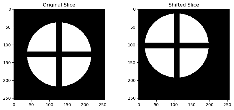
3. Batched Volume Warping

In X-ray tomography, we often calculate a shift or rotation on a single projection or slice and want to apply it to the entire stack efficiently. warp_volume_xy_batched handles this by applying a 2D matrix to every slice in a 3D volume, processing them in chunks to manage memory.

# Create a stack of identical images
stack_ref = np.repeat(ref_np[np.newaxis, :, :], 50, axis=0) # 50 slices

# Define a transformation matrix (Pixel space, like from Skimage/PyStackReg)
# Let's say we detected a shift of 10 pixels right and 5 pixels down
shift_x_pixels = 20
shift_y_pixels = 25
H, W = stack_ref.shape[1:]

# Pixel space affine matrix (3x3)
affine_pixel = np.array([
    [1, 0, shift_x_pixels],
    [0, 1, shift_y_pixels],
    [0, 0, 1]
])

print(f"Applying pixel shift ({shift_x_pixels}, {shift_y_pixels}) to stack of shape {stack_ref.shape}...")

# Apply to whole stack
warped_stack = reg.warp_volume_xy_batched(
    stack_ref,
    affine_matrix=affine_pixel,
    is_pixel_space=True, # Important: Tell function this is NOT normalized [-1, 1]
    batch_size=16,
    device=device
)

# Check result on one slice
plt.figure(figsize=(10, 4))
plt.subplot(121); plt.imshow(stack_ref[0], cmap='gray'); plt.title("Original Slice")
plt.subplot(122); plt.imshow(warped_stack[0], cmap='gray'); plt.title("Shifted Slice")
plt.show()

Applying pixel shift (20, 25) to stack of shape (50, 256, 256)...

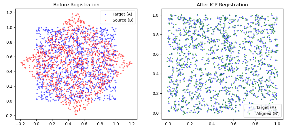
4. Point Cloud Registration (ICP)

Sometimes we deal with geometric data (coordinates) rather than pixel grids. icp_torch performs rigid registration on point clouds.

We will generate a random point cloud, rotate and translate it, and then recover the alignment.

# --- 1. Generate Point Clouds ---
num_points = 1000
# Source points (Model)
A = np.random.rand(num_points, 3).astype(np.float32)

# Create Target points (Data) by applying rigid transform
theta = np.radians(45)
R_gt = np.array([
    [np.cos(theta), -np.sin(theta), 0],
    [np.sin(theta),  np.cos(theta), 0],
    [0, 0, 1]
])
t_gt = np.array([0.5, -0.2, 0.1])

# B = A * R^T + t
B = A @ R_gt.T + t_gt

# Add some noise
B += np.random.normal(0, 0.01, B.shape)

# --- 2. Run ICP ---
print("Running ICP...")
B_aligned, R_est, t_est = reg.icp_torch(
    A, B,
    max_iterations=1000,
    lr=0.01,
    verbose=False
)

# --- 3. Visualization ---
# Project to 2D for plotting
plt.figure(figsize=(12, 5))

plt.subplot(121)
plt.scatter(A[:,0], A[:,1], s=5, c='blue', alpha=0.5, label='Target (A)')
plt.scatter(B[:,0], B[:,1], s=5, c='red', alpha=0.5, label='Source (B)')
plt.title("Before Registration")
plt.legend()

plt.subplot(122)
plt.scatter(A[:,0], A[:,1], s=5, c='blue', alpha=0.5, label='Target (A)')
plt.scatter(B_aligned[:,0], B_aligned[:,1], s=5, c='green', alpha=0.5, label='Aligned (B\')')
plt.title("After ICP Registration")
plt.legend()

plt.show()

print("Rotation Error (Frobenius):", np.linalg.norm(R_gt - R_est))
print("Translation Error:", np.linalg.norm(t_gt - t_est))

Running ICP...

Rotation Error (Frobenius): 2.0039074915494455
Translation Error: 1.0164983104253222

Summary of Key Takeaways

In this tutorial, we demonstrated how the ``reg_torch`` module provides a powerful, functional interface for geometric transformations and alignment within the nDTomo framework.

Key highlights include:

• Differentiable Alignment: By using PyTorch’s grid_sample and affine_grid, we can treat geometric parameters (rotation, translation, shear) as learnable weights, optimizing them via gradient descent rather than traditional search methods.

• Unified 2D & 3D Support: The library seamlessly handles both 2D image registration and 3D volumetric alignment using a consistent API.

• Batch Processing: We showed how to apply transformations efficiently to large stacks of data (e.g., laminography or tomography projections) using batched operations, essential for high-throughput pipelines.

• GPU Acceleration: All operations run natively on CUDA devices, enabling real-time performance even for complex 3D optimizations.

🚀 What You Can Do Next:

• Motion Correction in Tomography: Integrate register_affine_2d into a reconstruction loop to correct for sample drift or vibrations in experimental data before backprojection.

• Multimodal Registration: Use the ncc_loss (Normalized Cross Correlation) to align data from different modalities (e.g., X-ray fluorescence vs. diffraction contrast) where intensities may not be directly comparable.

Just like the reconstruction modules, these registration tools are designed to be modular and functional, empowering you to build custom, high-performance imaging pipelines without getting bogged down in complex class hierarchies.

This notebook serves as a foundation for building robust, motion-aware imaging workflows in nDTomo.