Direct Least Squares Reconstruction (DLSR) for XRD-CT Using PyTorch
📝 Introduction
This notebook provides the first open-source implementation of the Direct Least Squares Reconstruction (DLSR) method for X-ray diffraction computed tomography (XRD-CT), implemented entirely in Python using PyTorch with GPU acceleration.
Originally developed and validated using the TOPAS software, DLSR was introduced to solve the parallax artefact in XRD-CT (see Vamvakeros et al., J. Appl. Cryst., 53, 1531-1541, 2020, https://doi.org/10.1107/S1600576720013576) — a distortion that arises from the depth-dependent shift of Bragg peaks during pencil-beam scanning. Unlike filtered back projection (FBP), which reconstructs image intensities and then fits peaks post hoc, DLSR inverts the full forward model directly in parameter space (e.g., peak position, width, amplitude, background), yielding artefact-free maps in a single optimisation step.
Here, we extend the original work by:
Providing a fully open-source PyTorch-based implementation
Introducing a neural network model in place of voxel-wise parameter maps
Demonstrating improved performance under angular undersampling conditions
🎯 Objectives
By the end of this notebook, you will:
Understand the principle of DLSR and how it differs from conventional FBP-based pipelines
See how a neural network can be trained to directly reconstruct physical parameter maps from sinogram data
Compare the results of DLSR to FBP followed by post-reconstruction peak fitting
Evaluate the robustness of DLSR in cases of angular undersampling (e.g. few projection angles)
🧪 Why DLSR?
In conventional XRD-CT workflows:
The sinogram is reconstructed (e.g. via FBP)
Each voxel’s spectrum is then peak-fitted individually
This approach introduces errors if peak shapes or positions are misrepresented due to reconstruction artefacts (especially under parallax or sparse-angle sampling).
DLSR bypasses this problem by:
Treating peak parameters as the direct image to be reconstructed
Using the known physical forward model to generate sinograms from these parameters
Optimising parameter values by minimizing the difference between synthetic and experimental sinograms
📦 Dataset & Setup
This notebook uses synthetic data representing a 2D phantom with spatially varying peak parameters. The volume is forward-projected to create a sinogram, to which Poisson noise is added.
We then:
Train a PyTorch model to reconstruct the parameter maps directly from the sinogram
Compare DLSR output against conventional FBP + peak fitting
Explore reconstruction accuracy under angular undersampling
Let’s begin by importing the relevant packages and generating the dataset.
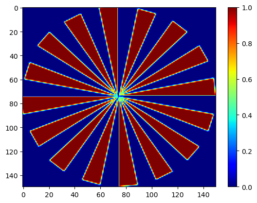
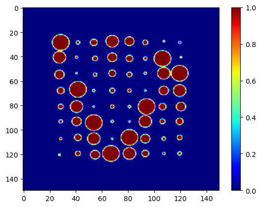
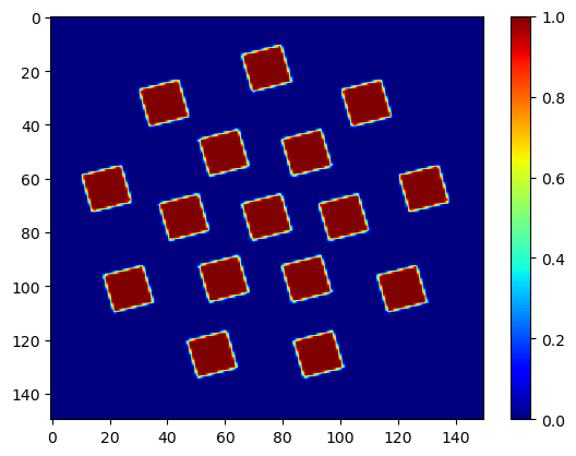
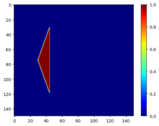
🧪 Generate Synthetic XRD-CT Phantom and 3D Hyperspectral Volume
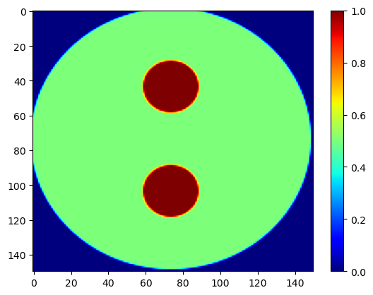
We begin by constructing a synthetic 2D spatial phantom composed of five components. These spatial maps (im1–im5) are used to define the spatially varying parameters of a single diffraction peak with linear background.
🏗️ Steps:
Define the diffraction domain:
The variable
xrepresents the diffraction axis (e.g., 2θ or q-space), sampled from 0 to 5 in steps of 0.25.
Assign parameter ranges:
peak_area,peak_position, andpeak_fwhmdefine the Gaussian peak.peak_slopeandpeak_interceptdefine the background.Each parameter is mapped from a phantom image and scaled linearly within its physical range.
Construct the volume:
A full 3D volume
volis generated where each voxel contains a 1D spectrum (Gaussian + linear background).Padding is applied around the spatial edges to avoid artefacts at boundaries.
Prepare for forward projection:
The volume is reshaped and converted into a PyTorch tensor (
yobs) on the GPU.Tensor dimensions are permuted into the expected format:
(batch, channels, height, width).
This synthetic dataset represents an ideal, ground-truth volume. It will later be forward-projected to simulate sinograms for DLSR training and evaluation.
[1]:
from nDTomo.sim.phantoms import load_example_patterns, nDTomophantom_2D, nDTomophantom_3D
from nDTomo.methods.plots import showspectra, showim
from nDTomo.methods.noise import addpnoise3D
from nDTomo.pytorch.tomo_torch import forward_project_3D
from nDTomo.pytorch.models_torch import PeakFitCNN, PrmCNN2D
from nDTomo.pytorch.utils_torch import calc_patches_indices, denormalize, filter_patch_indices, update_counter, initialize_counter, calc_patches_indices

import numpy as np
import matplotlib.pyplot as plt
from tqdm import tqdm
import torch, time
import torch.nn.functional as F
from torch import nn

# Create 2D spatial images for the five components
npix = 150
im1, im2, im3, im4, im5 = nDTomophantom_2D(npix, nim='Multiple')
iml = [im1, im2, im3, im4, im5]

im5 = im5/np.max(im5)

%matplotlib inline

# Optionally display spatial maps
showim(im1, 2)
showim(im2, 3)
showim(im3, 4)
showim(im4, 5)
showim(im5, 6)


def linear_background(x, slope, intercept):
    return slope*x + intercept

def gaussian(x, A, mu, sigma):
    return A * np.exp(-(x - mu)**2 / (2*sigma**2))

# Define the x axis
x = np.arange(0, 5, 0.25)

# Define the min/max for the various parameters

peak1_mu_min = 2
peak1_mu_max = 3

peak1_sigma_min = 0.2
peak1_sigma_max = 0.4

peak1_A_min = 0
peak1_A_max = 1.25

bkg_slope_min = 0.0
bkg_slope_max = 0.025

bkg_intercept_min = 0.05
bkg_intercept_max = 0.25

im6 = im2 + im5
im6 = im6 / np.max(im6)

peak_area = peak1_A_min + im6*(peak1_A_max - peak1_A_min)
peak_position = peak1_mu_min + im2*(peak1_mu_max - peak1_mu_min)
peak_fwhm = peak1_sigma_min + im3*(peak1_sigma_max - peak1_sigma_min)
peak_slope = bkg_slope_min + im4*(bkg_slope_max - bkg_slope_min)
peak_intercept = bkg_intercept_min + im5*(bkg_intercept_max - bkg_intercept_min)

vol = np.zeros((im1.shape[0], im1.shape[1], len(x)), dtype = 'float32')

mask_tmp = np.copy(peak_area)
mask_tmp[mask_tmp<0.0001] = 0
mask_tmp[mask_tmp>0] = 1

for ii in tqdm(range(im1.shape[0])):
    for jj in range(im1.shape[1]):
        if mask_tmp[ii,jj] > 0:
            vol[ii,jj,:] = gaussian(x, A=peak_area[ii,jj], mu=peak_position[ii,jj], sigma=peak_fwhm[ii,jj]) + \
                           linear_background(x, slope=peak_slope[ii,jj], intercept=peak_intercept[ii,jj])

extra = 5
vol = np.concatenate((np.zeros((vol.shape[0], extra, len(x)), dtype = 'float32'), vol, np.zeros((vol.shape[0], extra, len(x)), dtype = 'float32')), axis=1)
vol = np.concatenate((np.zeros((extra, vol.shape[1], len(x)), dtype = 'float32'), vol, np.zeros((extra, vol.shape[1], len(x)), dtype = 'float32')), axis=0)

print(vol.shape, np.max(vol))

volp = np.copy(vol)

yobs = np.transpose(volp, (2,1,0))
yobs = torch.tensor(yobs, dtype=torch.float32, device='cuda')
yobs = torch.reshape(yobs, (1, yobs.shape[0], yobs.shape[1], yobs.shape[2]))
yobs = torch.transpose(yobs, 3, 2)#[0,:,:,:]
print(yobs.shape)
c:\Users\anton\anaconda3\envs\ndtomo\lib\site-packages\h5py\__init__.py:36: UserWarning: h5py is running against HDF5 1.12.2 when it was built against 1.12.1, this may cause problems
  _warn(("h5py is running against HDF5 {0} when it was built against {1}, "
c:\Users\anton\anaconda3\envs\ndtomo\lib\site-packages\paramiko\pkey.py:82: CryptographyDeprecationWarning: TripleDES has been moved to cryptography.hazmat.decrepit.ciphers.algorithms.TripleDES and will be removed from this module in 48.0.0.
  "cipher": algorithms.TripleDES,
c:\Users\anton\anaconda3\envs\ndtomo\lib\site-packages\paramiko\transport.py:219: CryptographyDeprecationWarning: Blowfish has been moved to cryptography.hazmat.decrepit.ciphers.algorithms.Blowfish and will be removed from this module in 45.0.0.
  "class": algorithms.Blowfish,
c:\Users\anton\anaconda3\envs\ndtomo\lib\site-packages\paramiko\transport.py:243: CryptographyDeprecationWarning: TripleDES has been moved to cryptography.hazmat.decrepit.ciphers.algorithms.TripleDES and will be removed from this module in 48.0.0.
  "class": algorithms.TripleDES,
c:\Users\anton\anaconda3\envs\ndtomo\lib\site-packages\xdesign\geometry\area.py:789: UserWarning: Didn't check that Mesh contains Circle.
  warnings.warn("Didn't check that Mesh contains Circle.")
100%|██████████| 150/150 [00:00<00:00, 665.95it/s]
(160, 160, 20) 1.5
torch.Size([1, 20, 160, 160])
📡 Forward Project Synthetic Volume to Generate Noisy Sinogram
In this step, we simulate the experimental acquisition process by projecting the 3D synthetic volume onto a set of projection angles, thereby generating a sinogram volume. This sinogram volume will serve as the input to both the DLSR and FBP-based reconstruction pipelines.
🔧 Forward Projection
The
forward_project_3D()function computes parallel-beam projections of the hyperspectral volume (yobs) for a specified set of angles.Each projection corresponds to a linear integral along a direction in the
(x, y)plane, for each spectral channel.
Here we simulate:
A sparse angular acquisition using only
60projection angles between 0° and 180° (undersampled regime) for a sample that consists of150voxels in along one dimension (i.e. images consisting of150x150voxels)This mimics realistic conditions where scan time or radiation dose must be minimized.
🌫️ Add Poisson Noise
Poisson noise is added to the sinogram (
sn) usingaddpnoise3D()to emulate photon-counting statistics at moderate exposure (ct=100).
🔁 FBP Baseline (for Comparison)
As a baseline, we apply Filtered Back Projection (FBP) to the noisy sinogram using
astra_rec_vol().This yields a reconstructed hyperspectral volume (
r) from which conventional peak fitting will be performed later.
This step prepares both the noisy sinogram and its conventional reconstruction, which will serve as inputs for downstream analysis and comparisons.
[2]:
from nDTomo.tomo.astra_tomo import astra_rec_vol

angles = np.linspace(0, 180, 60, endpoint=False)

s = forward_project_3D(yobs, angles, npix=yobs.shape[2], nch=yobs.shape[1], device='cuda')

sn = s.cpu().detach().numpy()
sn = np.transpose(sn, (2,1,0))
sn = np.transpose(sn, (1,0,2))
sn = addpnoise3D(sn, ct=100)
print(s.shape)

r = astra_rec_vol(sn, theta=np.deg2rad(angles))
r[r<0] = 0
torch.Size([20, 160, 60])
100%|██████████| 20/20 [00:00<00:00, 24.60it/s]
🧠 Define Parameter Model for DLSR and Create Volume Mask
This section defines the parameter model used for DLSR reconstruction and prepares a spatial mask to constrain the optimisation.
🔧 Parameter Model (PrmCNN2D)
We use the PrmCNN2D module in parameter-map-only mode, where each peak and background parameter is initialized as a learnable 2D tensor:
num_peaks = 1→ Area, Position, FWHMBackground terms: Slope and Intercept
total_params = 5maps per voxel
The model holds npix × npix × total_params parameters, directly optimised to match observed sinogram projections.
This forms the core of the DLSR approach, where optimisation is done directly in parameter space.
🛡️ Circular Volume Mask
To avoid boundary artefacts and reduce overfitting at the edges:
A circular mask is applied to the 3D volume (
maskvol)This restricts the optimisation to the central region of the sample, which typically corresponds to valid illumination in experimental geometries
The helper function create_vol_mask():
Constructs a 3D binary mask using
cirmask()Applies it across all spectral channels
Converts it to a PyTorch tensor on the correct device
This mask will later be used to ensure that the DLSR loss is only computed in relevant regions of the volume.
[3]:
npix_x = volp.shape[0]
npix_y = volp.shape[1]
xv = torch.tensor(x, dtype=torch.float32, device='cuda')

### Single peak
peak_definitions = [(1, 1.0, 4.0)]

num_peaks = len(peak_definitions)
num_params_per_peak = 3  # Area, Position, FWHM
background_params = 2  # Slope, Intercept
total_params = num_peaks * num_params_per_peak + background_params

npix = volp.shape[0]
nch_in = total_params
nch_out = total_params
nfilts = 2*total_params # 2*total_params is pretty good when using norm layer
norm_type='layer'
activation='Sigmoid'
downsampling = 8
device = 'cuda'

model_prms_only = PrmCNN2D(npix, nch_in=nch_in, nch_out=nch_out, nfilts=nfilts, nlayers=1, norm_type='None',
               prms_layer=True, cnn_layer=False, tensor_vals = 'zeros').to(device)
model_prms = sum(p.numel() for p in model_prms_only.parameters() if p.requires_grad)
print(f"Total number of parameters: {model_prms}")
print("Conventional number of parameters:", npix*npix*total_params)

def cirmask(im, npx=0):
    """
    Apply a circular mask to the image
    """
    sz = np.floor(im.shape[0])
    x = np.arange(0,sz)
    x = np.tile(x,(int(sz),1))
    y = np.swapaxes(x,0,1)
    xc = np.round(sz/2)
    yc = np.round(sz/2)
    r = np.sqrt(((x-xc)**2 + (y-yc)**2));
    dim =  im.shape
    if len(dim)==2:
        im = np.where(r>np.floor(sz/2) - npx,0,im)
    elif len(dim)==3:
        for ii in range(0,dim[2]):
            im[:,:,ii] = np.where(r>np.floor(sz/2) - npx ,0,im[:,:,ii])
    return(im)

def create_vol_mask(npix, nbins, npx=0):
    mask = np.ones((npix, npix, nbins))
    mask = cirmask(mask,npx)
    mask = np.float32(mask)
    mask = np.transpose(mask, (2,1,0))
    mask = torch.from_numpy(mask)
    mask = torch.reshape(mask, (1, mask.shape[0], mask.shape[1], mask.shape[2]))
    mask = mask.to(device)
    return(mask)

maskvol = create_vol_mask(npix, len(x), npx=0)
print(maskvol.shape)
Total number of parameters: 128000
Conventional number of parameters: 128000
torch.Size([1, 20, 160, 160])
🔁 DLSR Training: Direct Least Squares Optimisation in Parameter Space
This section performs the core DLSR reconstruction. We directly optimise the peak and background parameter maps (stored in the PrmCNN2D model) to minimise the discrepancy between the experimental sinogram data and the forward projection of the estimated volume. We will call this the DLSR-prm approach.
🧠 Objective
Rather than reconstructing spectra and fitting peaks afterward (as in FBP), DLSR treats the parameters of the peak model as the image to be reconstructed. The pipeline:
Converts the predicted parameter maps into a synthetic volume via:
Gaussian peak generation
Linear background addition
Applies the same forward projection operator used to simulate the measured sinograms
Compares the synthetic sinograms (
s_gen) with the observed noisy (experimental) sinograms (s)Minimises the difference (RMSE) using gradient descent on the parameter maps
⚙️ Configuration
Parameter bounds (
param_min/param_max) constrain the optimization space for physical realismA soft clamp (±20%) is applied around the local average of each map to improve numerical stability during training
The reconstructed volume is masked using
maskvolto restrict fitting to valid regionsThe model is trained using PyTorch with GPU acceleration, using:
Adam optimizer
L1, MSE, and RMSE loss metrics (RMSE used for backprop)
ReduceLROnPlateauscheduler with early stopping
🔄 Training Loop Summary
For each epoch:
Reconstruct the 3D hyperspectral volume from the current parameter maps
Forward-project this volume into sinogram space
Compare with the observed sinogram
Update parameter maps via backpropagation
The loop stops automatically if the learning rate reaches its minimum value, or continues for up to 50,000 epochs.
📈 Output
At the end of training, the notebook prints:
Final values for MAE, MSE, and RMSE
Total number of epochs run
Total training time
This concludes the DLSR training stage, resulting in directly reconstructed peak parameter maps that we can now visualize and compare to conventional results.
[4]:
def gaussian(x, area, position, fwhm):
    """Gaussian peak shape."""
    return area * torch.exp(-(x - position)**2 / (2 * fwhm**2))

MAE = torch.nn.L1Loss()

### Single peak ###
param_min = {
    'Area': torch.zeros(num_peaks, dtype=torch.float32).to(device),
    'Position': torch.tensor([peak[1] for peak in peak_definitions], dtype=torch.float32).to(device),
    'FWHM': torch.zeros(num_peaks, dtype=torch.float32).to(device) + 0.1,
    'Fraction': torch.zeros(num_peaks, dtype=torch.float32).to(device),
    'Slope': torch.zeros(1, dtype=torch.float32).to(device),
    'Intercept': torch.zeros(1, dtype=torch.float32).to(device),
}
param_max = {
    'Area': torch.zeros(num_peaks, dtype=torch.float32).to(device) + 2,
    'Position': torch.tensor([peak[2] for peak in peak_definitions], dtype=torch.float32).to(device),
    'FWHM': torch.zeros(num_peaks, dtype=torch.float32).to(device) + 0.5,
    'Fraction': torch.zeros(num_peaks, dtype=torch.float32).to(device) + 1,
    'Slope': torch.zeros(1, dtype=torch.float32).to(device) + 0.2,
    'Intercept': torch.zeros(1, dtype=torch.float32).to(device) + 0.5,
}


nch = volp.shape[2]
im_static = np.sum(volp, axis=2)
im_static = im_static/np.max(im_static)
im_static = np.reshape(im_static, (1, 1, volp.shape[1], volp.shape[1]))
im_static = torch.tensor(im_static, dtype=torch.float32, device=device)

epochs = 2000
patience = 100 #250
min_lr = 1E-5
learning_rate = 0.1
optimizer = torch.optim.Adam(model_prms_only.parameters(), lr=learning_rate)
prf = 0.2
scheduler = torch.optim.lr_scheduler.ReduceLROnPlateau(optimizer, patience=patience, factor=0.5, min_lr=min_lr)

start = time.time()
logloss = []

for epoch in tqdm(range(epochs)):

    loss_acc = 0

    yc = model_prms_only(im_static)

    filtered = nn.AvgPool2d(kernel_size=3, stride=1, padding=1)(yc)
    lower_bound = filtered * (1 - prf)
    upper_bound = filtered * (1 + prf)
    yc = torch.clamp(yc, min=lower_bound, max=upper_bound)

    y = torch.zeros((npix*npix, len(xv)), dtype=torch.float32).to(device)
    for i in range(num_peaks):

        area = denormalize(yc[:, i * 3, :, :], 'Area', param_min, param_max, i)
        position = denormalize(yc[:, i * 3 + 1, :, :], 'Position', param_min, param_max, i)
        fwhm = denormalize(yc[:, i * 3 + 2, :, :], 'FWHM', param_min, param_max, i)

        area = torch.transpose(torch.reshape(area, (area.shape[0], area.shape[1]*area.shape[2])), 1, 0)
        position = torch.transpose(torch.reshape(position, (position.shape[0], position.shape[1]*position.shape[2])), 1, 0)
        fwhm = torch.transpose(torch.reshape(fwhm, (fwhm.shape[0], fwhm.shape[1]*fwhm.shape[2])), 1, 0)

        area = torch.reshape(area, (area.shape[0]*area.shape[1], 1))
        position = torch.reshape(position, (area.shape[0]*area.shape[1], 1))
        fwhm = torch.reshape(fwhm, (area.shape[0]*area.shape[1], 1))

        y += gaussian(xv.unsqueeze(0), area, position, fwhm)

    slope = denormalize(yc[:, -2, :, :], 'Slope', param_min, param_max, )
    intercept = denormalize(yc[:, -1, :, :], 'Intercept', param_min, param_max, )

    slope = torch.transpose(torch.reshape(slope, (slope.shape[0], slope.shape[1]*slope.shape[2])), 1, 0)
    intercept = torch.transpose(torch.reshape(intercept, (intercept.shape[0], intercept.shape[1]*intercept.shape[2])), 1, 0)

    slope = torch.reshape(slope, (slope.shape[0]*slope.shape[1], 1))
    intercept = torch.reshape(intercept, (intercept.shape[0]*intercept.shape[1], 1))

    y += slope * xv + intercept
    y = torch.reshape(y, (1, npix, npix, nch))
    y = torch.transpose(y, 3, 1)
    y = torch.transpose(y, 3, 2)
    y = y*maskvol

    s_gen = forward_project_3D(y, angles, npix=yobs.shape[2], nch=yobs.shape[1], device='cuda')

    loss_mae =  MAE(s, s_gen)
    loss_mse = torch.mean((s - s_gen) ** 2)
    loss_rmse = torch.sqrt(torch.mean((s - s_gen) ** 2))

    loss = loss_rmse
    optimizer.zero_grad()
    loss.backward()

    optimizer.step()

    logloss.append(loss.cpu().detach().numpy())

    scheduler.step(logloss[-1])

    if epoch %  (int(patience/2)) == 0:
        print('MAE = ', loss_mae, 'MSE = ', loss_mse,'RMSE = ', loss_rmse)
        print('Accumulated Loss = ', logloss[-1])

    if optimizer.param_groups[0]['lr'] == scheduler.min_lrs[0]:
        print("Minimum learning rate reached, stopping the optimization")
        print(epoch)
        break

total_time = time.time() - start

print(epoch, loss_mae, loss_mse, loss_rmse, logloss[-1])
print(total_time)
0%| | 2/2000 [00:00<02:15, 14.72it/s]
MAE =  tensor(56.6280, device='cuda:0', grad_fn=<MeanBackward0>) MSE =  tensor(4976.3975, device='cuda:0', grad_fn=<MeanBackward0>) RMSE =  tensor(70.5436, device='cuda:0', grad_fn=<SqrtBackward0>)
Accumulated Loss =  70.54359
3%|▎ | 54/2000 [00:03<01:56, 16.72it/s]
MAE =  tensor(4.2742, device='cuda:0', grad_fn=<MeanBackward0>) MSE =  tensor(36.4051, device='cuda:0', grad_fn=<MeanBackward0>) RMSE =  tensor(6.0337, device='cuda:0', grad_fn=<SqrtBackward0>)
Accumulated Loss =  6.0336614
5%|▌ | 104/2000 [00:06<01:45, 18.01it/s]
MAE =  tensor(1.2222, device='cuda:0', grad_fn=<MeanBackward0>) MSE =  tensor(2.4229, device='cuda:0', grad_fn=<MeanBackward0>) RMSE =  tensor(1.5566, device='cuda:0', grad_fn=<SqrtBackward0>)
Accumulated Loss =  1.5565635
8%|▊ | 153/2000 [00:08<01:44, 17.62it/s]
MAE =  tensor(0.6587, device='cuda:0', grad_fn=<MeanBackward0>) MSE =  tensor(0.7948, device='cuda:0', grad_fn=<MeanBackward0>) RMSE =  tensor(0.8915, device='cuda:0', grad_fn=<SqrtBackward0>)
Accumulated Loss =  0.89152044
10%|█ | 203/2000 [00:11<01:43, 17.42it/s]
MAE =  tensor(0.4756, device='cuda:0', grad_fn=<MeanBackward0>) MSE =  tensor(0.4344, device='cuda:0', grad_fn=<MeanBackward0>) RMSE =  tensor(0.6591, device='cuda:0', grad_fn=<SqrtBackward0>)
Accumulated Loss =  0.6591266
13%|█▎ | 254/2000 [00:14<01:46, 16.42it/s]
MAE =  tensor(0.3855, device='cuda:0', grad_fn=<MeanBackward0>) MSE =  tensor(0.2997, device='cuda:0', grad_fn=<MeanBackward0>) RMSE =  tensor(0.5474, device='cuda:0', grad_fn=<SqrtBackward0>)
Accumulated Loss =  0.547444
15%|█▌ | 302/2000 [00:17<01:48, 15.65it/s]
MAE =  tensor(0.3232, device='cuda:0', grad_fn=<MeanBackward0>) MSE =  tensor(0.2234, device='cuda:0', grad_fn=<MeanBackward0>) RMSE =  tensor(0.4726, device='cuda:0', grad_fn=<SqrtBackward0>)
Accumulated Loss =  0.47262138
18%|█▊ | 354/2000 [00:20<01:37, 16.94it/s]
MAE =  tensor(0.2929, device='cuda:0', grad_fn=<MeanBackward0>) MSE =  tensor(0.1897, device='cuda:0', grad_fn=<MeanBackward0>) RMSE =  tensor(0.4355, device='cuda:0', grad_fn=<SqrtBackward0>)
Accumulated Loss =  0.43553096
20%|██ | 403/2000 [00:23<01:30, 17.66it/s]
MAE =  tensor(0.2718, device='cuda:0', grad_fn=<MeanBackward0>) MSE =  tensor(0.1667, device='cuda:0', grad_fn=<MeanBackward0>) RMSE =  tensor(0.4082, device='cuda:0', grad_fn=<SqrtBackward0>)
Accumulated Loss =  0.40823066
23%|██▎ | 453/2000 [00:26<01:31, 16.88it/s]
MAE =  tensor(0.2469, device='cuda:0', grad_fn=<MeanBackward0>) MSE =  tensor(0.1437, device='cuda:0', grad_fn=<MeanBackward0>) RMSE =  tensor(0.3791, device='cuda:0', grad_fn=<SqrtBackward0>)
Accumulated Loss =  0.37908888
25%|██▌ | 504/2000 [00:29<01:32, 16.15it/s]
MAE =  tensor(0.2257, device='cuda:0', grad_fn=<MeanBackward0>) MSE =  tensor(0.1257, device='cuda:0', grad_fn=<MeanBackward0>) RMSE =  tensor(0.3546, device='cuda:0', grad_fn=<SqrtBackward0>)
Accumulated Loss =  0.35458285
28%|██▊ | 554/2000 [00:32<01:26, 16.68it/s]
MAE =  tensor(0.2202, device='cuda:0', grad_fn=<MeanBackward0>) MSE =  tensor(0.1218, device='cuda:0', grad_fn=<MeanBackward0>) RMSE =  tensor(0.3490, device='cuda:0', grad_fn=<SqrtBackward0>)
Accumulated Loss =  0.3489579
30%|███ | 604/2000 [00:35<01:24, 16.48it/s]
MAE =  tensor(0.2218, device='cuda:0', grad_fn=<MeanBackward0>) MSE =  tensor(0.1239, device='cuda:0', grad_fn=<MeanBackward0>) RMSE =  tensor(0.3521, device='cuda:0', grad_fn=<SqrtBackward0>)
Accumulated Loss =  0.35206524
33%|███▎ | 654/2000 [00:38<01:20, 16.76it/s]
MAE =  tensor(0.2079, device='cuda:0', grad_fn=<MeanBackward0>) MSE =  tensor(0.1132, device='cuda:0', grad_fn=<MeanBackward0>) RMSE =  tensor(0.3364, device='cuda:0', grad_fn=<SqrtBackward0>)
Accumulated Loss =  0.3364454
35%|███▌ | 704/2000 [00:41<01:17, 16.82it/s]
MAE =  tensor(0.1995, device='cuda:0', grad_fn=<MeanBackward0>) MSE =  tensor(0.1075, device='cuda:0', grad_fn=<MeanBackward0>) RMSE =  tensor(0.3279, device='cuda:0', grad_fn=<SqrtBackward0>)
Accumulated Loss =  0.3278623
38%|███▊ | 752/2000 [00:44<01:14, 16.77it/s]
MAE =  tensor(0.1939, device='cuda:0', grad_fn=<MeanBackward0>) MSE =  tensor(0.1039, device='cuda:0', grad_fn=<MeanBackward0>) RMSE =  tensor(0.3223, device='cuda:0', grad_fn=<SqrtBackward0>)
Accumulated Loss =  0.32229087
40%|████ | 804/2000 [00:47<01:12, 16.61it/s]
MAE =  tensor(0.1921, device='cuda:0', grad_fn=<MeanBackward0>) MSE =  tensor(0.1032, device='cuda:0', grad_fn=<MeanBackward0>) RMSE =  tensor(0.3213, device='cuda:0', grad_fn=<SqrtBackward0>)
Accumulated Loss =  0.3212524
43%|████▎ | 854/2000 [00:50<01:04, 17.91it/s]
MAE =  tensor(0.1852, device='cuda:0', grad_fn=<MeanBackward0>) MSE =  tensor(0.0988, device='cuda:0', grad_fn=<MeanBackward0>) RMSE =  tensor(0.3144, device='cuda:0', grad_fn=<SqrtBackward0>)
Accumulated Loss =  0.31436902
45%|████▌ | 904/2000 [00:53<01:02, 17.61it/s]
MAE =  tensor(0.1841, device='cuda:0', grad_fn=<MeanBackward0>) MSE =  tensor(0.0981, device='cuda:0', grad_fn=<MeanBackward0>) RMSE =  tensor(0.3132, device='cuda:0', grad_fn=<SqrtBackward0>)
Accumulated Loss =  0.31324595
48%|████▊ | 954/2000 [00:56<00:57, 18.10it/s]
MAE =  tensor(0.1854, device='cuda:0', grad_fn=<MeanBackward0>) MSE =  tensor(0.0987, device='cuda:0', grad_fn=<MeanBackward0>) RMSE =  tensor(0.3142, device='cuda:0', grad_fn=<SqrtBackward0>)
Accumulated Loss =  0.31415233
50%|█████ | 1004/2000 [00:59<00:58, 16.99it/s]
MAE =  tensor(0.1839, device='cuda:0', grad_fn=<MeanBackward0>) MSE =  tensor(0.0990, device='cuda:0', grad_fn=<MeanBackward0>) RMSE =  tensor(0.3146, device='cuda:0', grad_fn=<SqrtBackward0>)
Accumulated Loss =  0.31459925
53%|█████▎ | 1053/2000 [01:01<00:56, 16.84it/s]
MAE =  tensor(0.1787, device='cuda:0', grad_fn=<MeanBackward0>) MSE =  tensor(0.0956, device='cuda:0', grad_fn=<MeanBackward0>) RMSE =  tensor(0.3092, device='cuda:0', grad_fn=<SqrtBackward0>)
Accumulated Loss =  0.3091589
55%|█████▌ | 1104/2000 [01:04<00:49, 17.97it/s]
MAE =  tensor(0.1795, device='cuda:0', grad_fn=<MeanBackward0>) MSE =  tensor(0.0961, device='cuda:0', grad_fn=<MeanBackward0>) RMSE =  tensor(0.3100, device='cuda:0', grad_fn=<SqrtBackward0>)
Accumulated Loss =  0.30995244
58%|█████▊ | 1154/2000 [01:07<00:49, 17.13it/s]
MAE =  tensor(0.1752, device='cuda:0', grad_fn=<MeanBackward0>) MSE =  tensor(0.0937, device='cuda:0', grad_fn=<MeanBackward0>) RMSE =  tensor(0.3061, device='cuda:0', grad_fn=<SqrtBackward0>)
Accumulated Loss =  0.30609193
60%|██████ | 1203/2000 [01:10<00:48, 16.31it/s]
MAE =  tensor(0.1710, device='cuda:0', grad_fn=<MeanBackward0>) MSE =  tensor(0.0909, device='cuda:0', grad_fn=<MeanBackward0>) RMSE =  tensor(0.3015, device='cuda:0', grad_fn=<SqrtBackward0>)
Accumulated Loss =  0.3015271
63%|██████▎ | 1253/2000 [01:13<00:40, 18.36it/s]
MAE =  tensor(0.1709, device='cuda:0', grad_fn=<MeanBackward0>) MSE =  tensor(0.0905, device='cuda:0', grad_fn=<MeanBackward0>) RMSE =  tensor(0.3008, device='cuda:0', grad_fn=<SqrtBackward0>)
Accumulated Loss =  0.30076694
65%|██████▌ | 1304/2000 [01:16<00:43, 16.06it/s]
MAE =  tensor(0.1688, device='cuda:0', grad_fn=<MeanBackward0>) MSE =  tensor(0.0893, device='cuda:0', grad_fn=<MeanBackward0>) RMSE =  tensor(0.2989, device='cuda:0', grad_fn=<SqrtBackward0>)
Accumulated Loss =  0.2988817
68%|██████▊ | 1353/2000 [01:19<00:38, 16.93it/s]
MAE =  tensor(0.1696, device='cuda:0', grad_fn=<MeanBackward0>) MSE =  tensor(0.0897, device='cuda:0', grad_fn=<MeanBackward0>) RMSE =  tensor(0.2996, device='cuda:0', grad_fn=<SqrtBackward0>)
Accumulated Loss =  0.29955056
70%|███████ | 1403/2000 [01:22<00:32, 18.37it/s]
MAE =  tensor(0.1690, device='cuda:0', grad_fn=<MeanBackward0>) MSE =  tensor(0.0904, device='cuda:0', grad_fn=<MeanBackward0>) RMSE =  tensor(0.3006, device='cuda:0', grad_fn=<SqrtBackward0>)
Accumulated Loss =  0.3006343
73%|███████▎ | 1453/2000 [01:25<00:32, 16.97it/s]
MAE =  tensor(0.1643, device='cuda:0', grad_fn=<MeanBackward0>) MSE =  tensor(0.0868, device='cuda:0', grad_fn=<MeanBackward0>) RMSE =  tensor(0.2946, device='cuda:0', grad_fn=<SqrtBackward0>)
Accumulated Loss =  0.29455084
75%|███████▌ | 1504/2000 [01:28<00:28, 17.44it/s]
MAE =  tensor(0.1670, device='cuda:0', grad_fn=<MeanBackward0>) MSE =  tensor(0.0882, device='cuda:0', grad_fn=<MeanBackward0>) RMSE =  tensor(0.2970, device='cuda:0', grad_fn=<SqrtBackward0>)
Accumulated Loss =  0.29699236
78%|███████▊ | 1554/2000 [01:31<00:27, 16.08it/s]
MAE =  tensor(0.1665, device='cuda:0', grad_fn=<MeanBackward0>) MSE =  tensor(0.0891, device='cuda:0', grad_fn=<MeanBackward0>) RMSE =  tensor(0.2985, device='cuda:0', grad_fn=<SqrtBackward0>)
Accumulated Loss =  0.2985142
80%|████████ | 1603/2000 [01:34<00:22, 17.49it/s]
MAE =  tensor(0.1556, device='cuda:0', grad_fn=<MeanBackward0>) MSE =  tensor(0.0817, device='cuda:0', grad_fn=<MeanBackward0>) RMSE =  tensor(0.2859, device='cuda:0', grad_fn=<SqrtBackward0>)
Accumulated Loss =  0.28589728
83%|████████▎ | 1654/2000 [01:37<00:19, 17.77it/s]
MAE =  tensor(0.1550, device='cuda:0', grad_fn=<MeanBackward0>) MSE =  tensor(0.0814, device='cuda:0', grad_fn=<MeanBackward0>) RMSE =  tensor(0.2853, device='cuda:0', grad_fn=<SqrtBackward0>)
Accumulated Loss =  0.2852763
85%|████████▌ | 1704/2000 [01:40<00:17, 17.20it/s]
MAE =  tensor(0.1546, device='cuda:0', grad_fn=<MeanBackward0>) MSE =  tensor(0.0812, device='cuda:0', grad_fn=<MeanBackward0>) RMSE =  tensor(0.2849, device='cuda:0', grad_fn=<SqrtBackward0>)
Accumulated Loss =  0.2849102
88%|████████▊ | 1753/2000 [01:43<00:14, 17.46it/s]
MAE =  tensor(0.1542, device='cuda:0', grad_fn=<MeanBackward0>) MSE =  tensor(0.0810, device='cuda:0', grad_fn=<MeanBackward0>) RMSE =  tensor(0.2846, device='cuda:0', grad_fn=<SqrtBackward0>)
Accumulated Loss =  0.2845791
90%|█████████ | 1803/2000 [01:46<00:11, 17.05it/s]
MAE =  tensor(0.1538, device='cuda:0', grad_fn=<MeanBackward0>) MSE =  tensor(0.0808, device='cuda:0', grad_fn=<MeanBackward0>) RMSE =  tensor(0.2842, device='cuda:0', grad_fn=<SqrtBackward0>)
Accumulated Loss =  0.2842484
93%|█████████▎| 1853/2000 [01:49<00:08, 16.91it/s]
MAE =  tensor(0.1534, device='cuda:0', grad_fn=<MeanBackward0>) MSE =  tensor(0.0806, device='cuda:0', grad_fn=<MeanBackward0>) RMSE =  tensor(0.2839, device='cuda:0', grad_fn=<SqrtBackward0>)
Accumulated Loss =  0.28393552
95%|█████████▌| 1904/2000 [01:51<00:05, 17.42it/s]
MAE =  tensor(0.1531, device='cuda:0', grad_fn=<MeanBackward0>) MSE =  tensor(0.0804, device='cuda:0', grad_fn=<MeanBackward0>) RMSE =  tensor(0.2836, device='cuda:0', grad_fn=<SqrtBackward0>)
Accumulated Loss =  0.28359103
98%|█████████▊| 1953/2000 [01:54<00:02, 18.25it/s]
MAE =  tensor(0.1527, device='cuda:0', grad_fn=<MeanBackward0>) MSE =  tensor(0.0802, device='cuda:0', grad_fn=<MeanBackward0>) RMSE =  tensor(0.2833, device='cuda:0', grad_fn=<SqrtBackward0>)
Accumulated Loss =  0.2832709
100%|██████████| 2000/2000 [01:57<00:00, 17.03it/s]
1999 tensor(0.1524, device='cuda:0', grad_fn=<MeanBackward0>) tensor(0.0801, device='cuda:0', grad_fn=<MeanBackward0>) tensor(0.2830, device='cuda:0', grad_fn=<SqrtBackward0>) 0.28297925
117.42828679084778
🧪 Visualize and Compare DLSR Parameter Maps to Ground Truth
After training, we now extract the final parameter maps from the DLSR model and compare them to the original synthetic ground truth.
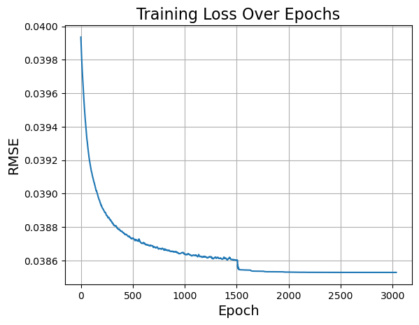
📉 Loss Curve
First, we plot the training loss (logloss) from epoch 100 onward to visually confirm convergence and stability of the DLSR optimisation.
🗺️ Extract Predicted Parameter Maps
We apply a final forward pass to extract the predicted maps for:
Peak Area
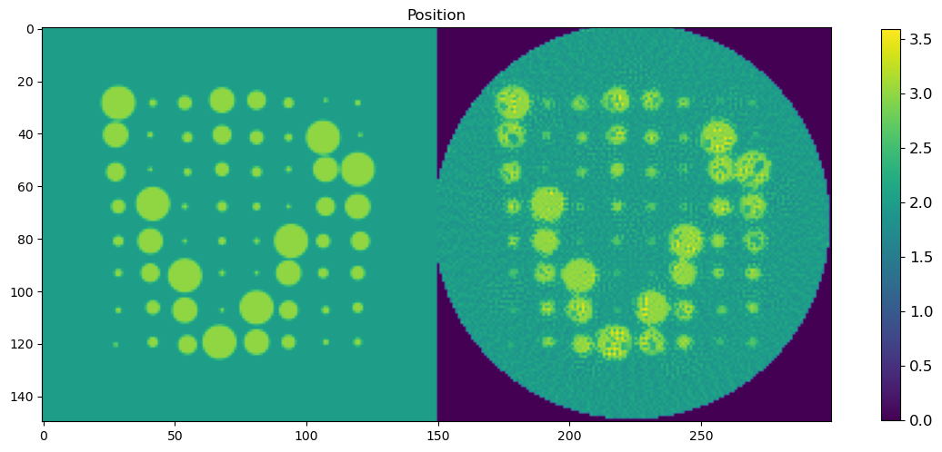
Peak Position
Peak FWHM
Background Slope
Background Intercept
The predicted maps are clamped using local smoothing and then denormalized to recover physical units.
To correct for padding added earlier, we crop the predicted maps to match the ground truth shape using an offset (ofs).
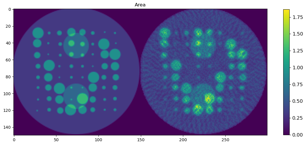
🎯 Comparison Strategy
To evaluate reconstruction quality:
A binary mask is applied (
msk) to ignore background regionsEach predicted map is concatenated with its corresponding ground truth map along the horizontal axis
This creates composite images where:
Left half = Ground truth
Right half = DLSR prediction (masked)
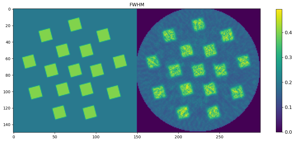
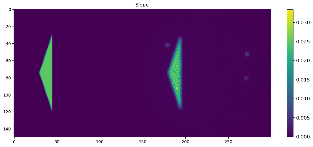
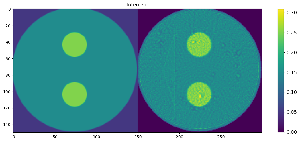
🖼️ Display Results
We visualize all five parameter maps using imshow():
Peak Area
Peak Position
Peak FWHM
Background Slope
Background Intercept
This visual comparison highlights the spatial accuracy and denoising capabilities of the DLSR approach under angular undersampling.
[29]:
%matplotlib inline

plt.figure(1);plt.clf()
plt.plot(logloss[100:])
plt.xlabel('Epoch', fontsize=14)
plt.ylabel('RMSE', fontsize=14)
plt.title('Training Loss Over Epochs', fontsize=16)
plt.grid(True)
plt.show()

ims = model_prms_only(im_static)
filtered = nn.AvgPool2d(kernel_size=5, stride=1, padding=2)(ims)
lower_bound = filtered * (1 - prf)
upper_bound = filtered * (1 + prf)
ims = torch.clamp(ims, min=lower_bound, max=upper_bound)

i = 0

prms_peak1_area = denormalize(ims[:, i * 3, :, :], 'Area', param_min, param_max, i)[0,:,:].cpu().detach().numpy()
prms_peak1_pos = denormalize(ims[:, i * 3 + 1, :, :], 'Position', param_min, param_max, i)[0,:,:].cpu().detach().numpy()
prms_peak1_fwhm = denormalize(ims[:, i * 3 + 2, :, :], 'FWHM', param_min, param_max, i)[0,:,:].cpu().detach().numpy()
prms_slope = denormalize(ims[:, -2, :, :], 'Slope', param_min, param_max, )[0,:,:].cpu().detach().numpy()
prms_intercept = denormalize(ims[:, -1, :, :], 'Intercept', param_min, param_max, )[0,:,:].cpu().detach().numpy()

ofs = int((prms_peak1_area.shape[0] - peak_area.shape[0])/2)

prms_peak1_area_dlsr = prms_peak1_area[ofs:prms_peak1_area.shape[0]-ofs, ofs:prms_peak1_area.shape[1]-ofs]
prms_peak1_pos_dlsr = prms_peak1_pos[ofs:prms_peak1_pos.shape[0]-ofs, ofs:prms_peak1_pos.shape[1]-ofs]
prms_peak1_fwhm_dlsr = prms_peak1_fwhm[ofs:prms_peak1_fwhm.shape[0]-ofs, ofs:prms_peak1_fwhm.shape[1]-ofs]
prms_slope_dlsr = prms_slope[ofs:prms_slope.shape[0]-ofs, ofs:prms_slope.shape[1]-ofs]
prms_intercept_dlsr = prms_intercept[ofs:prms_intercept.shape[0]-ofs, ofs:prms_intercept.shape[1]-ofs]

msk = np.copy(peak_area)
msk[msk<0.1] = 0
msk[msk>0] = 1

areac = np.concatenate((peak_area, prms_peak1_area_dlsr*msk), axis = 1)
posc = np.concatenate((peak_position, prms_peak1_pos_dlsr*msk), axis = 1)
fwhmc = np.concatenate((peak_fwhm, prms_peak1_fwhm_dlsr*msk), axis = 1)
slopec = np.concatenate((peak_slope, prms_slope_dlsr*msk), axis = 1)
interceptc = np.concatenate((peak_intercept, prms_intercept_dlsr*msk), axis = 1)

plt.figure(1, figsize=(14,14));plt.clf()
h = plt.imshow(areac)
cbar = plt.colorbar(h, shrink=0.4)
cbar.ax.tick_params(labelsize=12)
plt.title('Area')
plt.show()

plt.figure(2, figsize=(14,14));plt.clf()
h = plt.imshow(posc)
cbar = plt.colorbar(h, shrink=0.4)
cbar.ax.tick_params(labelsize=12)
plt.title('Position')
plt.show()

plt.figure(3, figsize=(14,14));plt.clf()
h = plt.imshow(fwhmc)
cbar = plt.colorbar(h, shrink=0.4)
cbar.ax.tick_params(labelsize=12)
plt.title('FWHM')
plt.show()

plt.figure(4, figsize=(14,14));plt.clf()
h = plt.imshow(slopec)
cbar = plt.colorbar(h, shrink=0.4)
cbar.ax.tick_params(labelsize=12)
plt.title('Slope')
plt.show()

plt.figure(5, figsize=(14,14));plt.clf()
h = plt.imshow(interceptc)
cbar = plt.colorbar(h, shrink=0.4)
cbar.ax.tick_params(labelsize=12)
plt.title('Intercept')
plt.show()
🤖 Define PeakFitCNN Model for Comparison with DLSR-prm
To benchmark the performance of DLSR, we now set up a second approach based on self-supervised CNN-based peak fitting using the PeakFitCNN model. This method is introduced and validated in a separate notebook.
🧠 PeakFitCNN Overview
The CNN receives a 4× downsampled hyperspectral input volume.
It predicts full-resolution parameter maps for:
Peak area, position, FWHM
Background slope and intercept
These maps are later used to reconstruct the full volume, which can be forward-projected and compared to the original sinogram.
⚙️ Model Configuration
nch_in: number of diffraction channels (e.g., 20)nch_out: total number of output parameter maps (5 in this case)nfilts: number of filters, chosen here as equal to input channels for simplicityupscale_factor = 4: restores full resolution from the downsampled inputnorm_type = 'layer': uses layer normalization for stabilityactivation = 'Sigmoid': ensures output values are in [0, 1] before denormalization
The total number of trainable parameters is printed and compared to the parameter count used in the DLSR approach.
🔻 Input Preparation
The FBP reconstructed volume is reshaped into a 4D tensor compatible with PyTorch
It is then downsampled by a factor of 4 using bilinear interpolation
This downsampled input will be used to train PeakFitCNN in a self-supervised manner, mimicking limited-resolution experimental data. The upcoming training loop will mirror that used for DLSR but applied to this deep model.
[6]:
model_cnn = PeakFitCNN(nch_in=volp.shape[2], nch_out=nch_out, nfilts=32,  upscale_factor = 4, norm_type='layer',
              activation='Sigmoid', padding='same', npix = volp.shape[0]//4).to(device)


nch_in = volp.shape[2]
nfilts = volp.shape[2] # 2*total_params

# Calculate the total number of parameters
model_prms = sum(p.numel() for p in model_cnn.parameters() if p.requires_grad)
print(f"Total number of parameters: {model_prms}")

print('Number of filters:', nfilts)
print(nch_out)

print("Conventional number of parameters:", npix*npix*total_params)

print(volp.shape[0])

ylow = np.transpose(r, (2,1,0))
ylow = torch.tensor(ylow, dtype=torch.float32, device=device)
ylow = torch.reshape(ylow, (1, ylow.shape[0], ylow.shape[1], ylow.shape[2]))
ylow = torch.transpose(ylow, 3, 2)
downsampled = F.interpolate(ylow, scale_factor=1/4, mode='bilinear', align_corners=False)
print(downsampled.shape, yobs.shape, yobs.shape[2]/4)
Total number of parameters: 2073733
Number of filters: 20
5
Conventional number of parameters: 128000
160
torch.Size([1, 20, 40, 40]) torch.Size([1, 20, 160, 160]) 40.0
🔁 Train PeakFitCNN Using Self-Supervised Spectral Reconstruction
In this section, we train the PeakFitCNN model to reconstruct peak parameters directly from the downsampled hyperspectral input. The training follows the same self-supervised loss formulation as used in DLSR, where the forward projection of the predicted volume is matched against the observed sinogram.
🎯 Objective
Rather than optimizing parameter maps directly, as in DLSR, we now learn a convolutional model that:
Takes as input a low-resolution hyperspectral volume
Predicts full-resolution peak parameters
Minimizes the sinogram error via a differentiable forward model
🧠 Training Setup
param_minandparam_max: define valid physical ranges for each parameterprf = 0.2: soft constraint (±20%) around the local average to stabilize outputoptimizer: Adam with learning rate0.001scheduler: Reduces learning rate when validation loss plateausloss: RMSE between generated (s_gen) and true (s) sinograms
🔁 Training Loop
For each epoch:
Forward pass through
model_cnn(downsampled)Clamp and denormalize the predicted parameter maps
Reconstruct the full 3D volume from the predicted parameters
Apply forward projection to obtain a synthetic sinogram
Compute reconstruction error against the observed sinogram
Backpropagate and update model weights
The model is trained using end-to-end self-supervision, without any direct labels for peak parameters.
📈 Output
At the end of training, the notebook reports:
Final values for MAE, MSE, and RMSE
Number of epochs completed
Total training time in seconds
This completes the CNN-based reconstruction, which we will next compare visually and quantitatively against the DLSR solution.
[7]:
def gaussian(x, area, position, fwhm):
    """Gaussian peak shape."""
    return area * torch.exp(-(x - position)**2 / (2 * fwhm**2))

MAE = torch.nn.L1Loss()

### Single peak ###
param_min = {
    'Area': torch.zeros(num_peaks, dtype=torch.float32).to(device),
    'Position': torch.tensor([peak[1] for peak in peak_definitions], dtype=torch.float32).to(device),
    'FWHM': torch.zeros(num_peaks, dtype=torch.float32).to(device) + 0.1,
    'Fraction': torch.zeros(num_peaks, dtype=torch.float32).to(device),
    'Slope': torch.zeros(1, dtype=torch.float32).to(device),
    'Intercept': torch.zeros(1, dtype=torch.float32).to(device),
}
param_max = {
    'Area': torch.zeros(num_peaks, dtype=torch.float32).to(device) + 2,
    'Position': torch.tensor([peak[2] for peak in peak_definitions], dtype=torch.float32).to(device),
    'FWHM': torch.zeros(num_peaks, dtype=torch.float32).to(device) + 0.5,
    'Fraction': torch.zeros(num_peaks, dtype=torch.float32).to(device) + 1,
    'Slope': torch.zeros(1, dtype=torch.float32).to(device) + 0.2,
    'Intercept': torch.zeros(1, dtype=torch.float32).to(device) + 0.5,
}

epochs = 50000
patience = 50 #250
min_lr = 1E-5
learning_rate = 0.001
optimizer = torch.optim.Adam(model_cnn.parameters(), lr=learning_rate)
prf = 0.2
scheduler = torch.optim.lr_scheduler.ReduceLROnPlateau(optimizer, patience=patience, factor=0.5, min_lr=min_lr)

start = time.time()
logloss = []

for epoch in tqdm(range(epochs)):

    loss_acc = 0

    yc = model_cnn(downsampled)

    filtered = nn.AvgPool2d(kernel_size=3, stride=1, padding=1)(yc)
    lower_bound = filtered * (1 - prf)
    upper_bound = filtered * (1 + prf)
    yc = torch.clamp(yc, min=lower_bound, max=upper_bound)

    y = torch.zeros((npix*npix, len(xv)), dtype=torch.float32).to(device)
    for i in range(num_peaks):

        area = denormalize(yc[:, i * 3, :, :], 'Area', param_min, param_max, i)
        position = denormalize(yc[:, i * 3 + 1, :, :], 'Position', param_min, param_max, i)
        fwhm = denormalize(yc[:, i * 3 + 2, :, :], 'FWHM', param_min, param_max, i)

        area = torch.transpose(torch.reshape(area, (area.shape[0], area.shape[1]*area.shape[2])), 1, 0)
        position = torch.transpose(torch.reshape(position, (position.shape[0], position.shape[1]*position.shape[2])), 1, 0)
        fwhm = torch.transpose(torch.reshape(fwhm, (fwhm.shape[0], fwhm.shape[1]*fwhm.shape[2])), 1, 0)

        area = torch.reshape(area, (area.shape[0]*area.shape[1], 1))
        position = torch.reshape(position, (area.shape[0]*area.shape[1], 1))
        fwhm = torch.reshape(fwhm, (area.shape[0]*area.shape[1], 1))

        y += gaussian(xv.unsqueeze(0), area, position, fwhm)

    slope = denormalize(yc[:, -2, :, :], 'Slope', param_min, param_max, )
    intercept = denormalize(yc[:, -1, :, :], 'Intercept', param_min, param_max, )

    slope = torch.transpose(torch.reshape(slope, (slope.shape[0], slope.shape[1]*slope.shape[2])), 1, 0)
    intercept = torch.transpose(torch.reshape(intercept, (intercept.shape[0], intercept.shape[1]*intercept.shape[2])), 1, 0)

    slope = torch.reshape(slope, (slope.shape[0]*slope.shape[1], 1))
    intercept = torch.reshape(intercept, (intercept.shape[0]*intercept.shape[1], 1))

    y += slope * xv + intercept
    y = torch.reshape(y, (1, npix, npix, nch))
    y = torch.transpose(y, 3, 1)
    y = torch.transpose(y, 3, 2)

    y = y * maskvol
    s_gen = forward_project_3D(y, angles, npix=yobs.shape[2], nch=yobs.shape[1], device='cuda')


    loss_mae =  MAE(s, s_gen)
    loss_mse = torch.mean((s - s_gen) ** 2)
    loss_rmse = torch.sqrt(torch.mean((s - s_gen) ** 2))

    loss = loss_rmse
    optimizer.zero_grad()
    loss.backward()

    optimizer.step()

    logloss.append(loss.cpu().detach().numpy())

    scheduler.step(logloss[-1])

    if epoch % int(patience*2) == 0:
        print('MAE = ', loss_mae, 'MSE = ', loss_mse,'RMSE = ', loss_rmse)
        print('Accumulated Loss = ', logloss[-1])

    if optimizer.param_groups[0]['lr'] == scheduler.min_lrs[0]:
        print("Minimum learning rate reached, stopping the optimization")
        print(epoch)
        break

total_time = time.time() - start

print(epoch, loss_mae, loss_mse, loss_rmse, logloss[-1])
print(total_time)
0%| | 3/50000 [00:01<4:10:40, 3.32it/s]
MAE =  tensor(46.6050, device='cuda:0', grad_fn=<MeanBackward0>) MSE =  tensor(3656.2676, device='cuda:0', grad_fn=<MeanBackward0>) RMSE =  tensor(60.4671, device='cuda:0', grad_fn=<SqrtBackward0>)
Accumulated Loss =  60.46708
0%| | 103/50000 [00:07<53:17, 15.60it/s]
MAE =  tensor(2.9521, device='cuda:0', grad_fn=<MeanBackward0>) MSE =  tensor(25.5371, device='cuda:0', grad_fn=<MeanBackward0>) RMSE =  tensor(5.0534, device='cuda:0', grad_fn=<SqrtBackward0>)
Accumulated Loss =  5.053422
0%| | 203/50000 [00:14<57:12, 14.51it/s]
MAE =  tensor(1.9229, device='cuda:0', grad_fn=<MeanBackward0>) MSE =  tensor(10.0414, device='cuda:0', grad_fn=<MeanBackward0>) RMSE =  tensor(3.1688, device='cuda:0', grad_fn=<SqrtBackward0>)
Accumulated Loss =  3.1688225
1%| | 303/50000 [00:21<51:19, 16.14it/s]
MAE =  tensor(1.0203, device='cuda:0', grad_fn=<MeanBackward0>) MSE =  tensor(2.8094, device='cuda:0', grad_fn=<MeanBackward0>) RMSE =  tensor(1.6761, device='cuda:0', grad_fn=<SqrtBackward0>)
Accumulated Loss =  1.6761379
1%| | 403/50000 [00:27<51:04, 16.19it/s]
MAE =  tensor(0.8660, device='cuda:0', grad_fn=<MeanBackward0>) MSE =  tensor(1.7052, device='cuda:0', grad_fn=<MeanBackward0>) RMSE =  tensor(1.3058, device='cuda:0', grad_fn=<SqrtBackward0>)
Accumulated Loss =  1.3058243
1%| | 504/50000 [00:34<51:56, 15.88it/s]
MAE =  tensor(0.7409, device='cuda:0', grad_fn=<MeanBackward0>) MSE =  tensor(1.1888, device='cuda:0', grad_fn=<MeanBackward0>) RMSE =  tensor(1.0903, device='cuda:0', grad_fn=<SqrtBackward0>)
Accumulated Loss =  1.0903063
1%| | 602/50000 [00:40<58:22, 14.10it/s]
MAE =  tensor(0.6013, device='cuda:0', grad_fn=<MeanBackward0>) MSE =  tensor(0.8286, device='cuda:0', grad_fn=<MeanBackward0>) RMSE =  tensor(0.9103, device='cuda:0', grad_fn=<SqrtBackward0>)
Accumulated Loss =  0.9102559
1%|▏ | 703/50000 [00:47<55:44, 14.74it/s]
MAE =  tensor(0.5615, device='cuda:0', grad_fn=<MeanBackward0>) MSE =  tensor(0.7155, device='cuda:0', grad_fn=<MeanBackward0>) RMSE =  tensor(0.8458, device='cuda:0', grad_fn=<SqrtBackward0>)
Accumulated Loss =  0.84584945
2%|▏ | 803/50000 [00:53<50:28, 16.24it/s]
MAE =  tensor(0.4403, device='cuda:0', grad_fn=<MeanBackward0>) MSE =  tensor(0.4648, device='cuda:0', grad_fn=<MeanBackward0>) RMSE =  tensor(0.6818, device='cuda:0', grad_fn=<SqrtBackward0>)
Accumulated Loss =  0.6817777
2%|▏ | 903/50000 [01:00<51:19, 15.94it/s]
MAE =  tensor(0.3954, device='cuda:0', grad_fn=<MeanBackward0>) MSE =  tensor(0.3598, device='cuda:0', grad_fn=<MeanBackward0>) RMSE =  tensor(0.5998, device='cuda:0', grad_fn=<SqrtBackward0>)
Accumulated Loss =  0.59984404
2%|▏ | 1003/50000 [01:06<53:30, 15.26it/s]
MAE =  tensor(0.3502, device='cuda:0', grad_fn=<MeanBackward0>) MSE =  tensor(0.2759, device='cuda:0', grad_fn=<MeanBackward0>) RMSE =  tensor(0.5253, device='cuda:0', grad_fn=<SqrtBackward0>)
Accumulated Loss =  0.52525663
2%|▏ | 1103/50000 [01:13<54:38, 14.92it/s]
MAE =  tensor(0.3072, device='cuda:0', grad_fn=<MeanBackward0>) MSE =  tensor(0.2178, device='cuda:0', grad_fn=<MeanBackward0>) RMSE =  tensor(0.4667, device='cuda:0', grad_fn=<SqrtBackward0>)
Accumulated Loss =  0.46670815
2%|▏ | 1203/50000 [01:20<51:17, 15.86it/s]
MAE =  tensor(0.2880, device='cuda:0', grad_fn=<MeanBackward0>) MSE =  tensor(0.1855, device='cuda:0', grad_fn=<MeanBackward0>) RMSE =  tensor(0.4307, device='cuda:0', grad_fn=<SqrtBackward0>)
Accumulated Loss =  0.4307308
3%|▎ | 1303/50000 [01:26<57:15, 14.17it/s]
MAE =  tensor(0.2662, device='cuda:0', grad_fn=<MeanBackward0>) MSE =  tensor(0.1623, device='cuda:0', grad_fn=<MeanBackward0>) RMSE =  tensor(0.4029, device='cuda:0', grad_fn=<SqrtBackward0>)
Accumulated Loss =  0.40287954
3%|▎ | 1403/50000 [01:33<50:44, 15.96it/s]
MAE =  tensor(0.2514, device='cuda:0', grad_fn=<MeanBackward0>) MSE =  tensor(0.1450, device='cuda:0', grad_fn=<MeanBackward0>) RMSE =  tensor(0.3807, device='cuda:0', grad_fn=<SqrtBackward0>)
Accumulated Loss =  0.38072848
3%|▎ | 1503/50000 [01:40<58:22, 13.85it/s]
MAE =  tensor(0.2393, device='cuda:0', grad_fn=<MeanBackward0>) MSE =  tensor(0.1317, device='cuda:0', grad_fn=<MeanBackward0>) RMSE =  tensor(0.3629, device='cuda:0', grad_fn=<SqrtBackward0>)
Accumulated Loss =  0.36286336
3%|▎ | 1603/50000 [01:46<53:07, 15.19it/s]
MAE =  tensor(0.2275, device='cuda:0', grad_fn=<MeanBackward0>) MSE =  tensor(0.1186, device='cuda:0', grad_fn=<MeanBackward0>) RMSE =  tensor(0.3443, device='cuda:0', grad_fn=<SqrtBackward0>)
Accumulated Loss =  0.34432393
3%|▎ | 1703/50000 [01:53<52:15, 15.40it/s]
MAE =  tensor(0.2169, device='cuda:0', grad_fn=<MeanBackward0>) MSE =  tensor(0.1073, device='cuda:0', grad_fn=<MeanBackward0>) RMSE =  tensor(0.3276, device='cuda:0', grad_fn=<SqrtBackward0>)
Accumulated Loss =  0.32763898
4%|▎ | 1803/50000 [02:00<1:00:40, 13.24it/s]
MAE =  tensor(0.2084, device='cuda:0', grad_fn=<MeanBackward0>) MSE =  tensor(0.0995, device='cuda:0', grad_fn=<MeanBackward0>) RMSE =  tensor(0.3154, device='cuda:0', grad_fn=<SqrtBackward0>)
Accumulated Loss =  0.31541568
4%|▍ | 1903/50000 [02:06<53:21, 15.02it/s]
MAE =  tensor(0.2004, device='cuda:0', grad_fn=<MeanBackward0>) MSE =  tensor(0.0925, device='cuda:0', grad_fn=<MeanBackward0>) RMSE =  tensor(0.3041, device='cuda:0', grad_fn=<SqrtBackward0>)
Accumulated Loss =  0.30406603
4%|▍ | 2003/50000 [02:13<55:45, 14.35it/s]
MAE =  tensor(0.1932, device='cuda:0', grad_fn=<MeanBackward0>) MSE =  tensor(0.0861, device='cuda:0', grad_fn=<MeanBackward0>) RMSE =  tensor(0.2935, device='cuda:0', grad_fn=<SqrtBackward0>)
Accumulated Loss =  0.29350188
4%|▍ | 2103/50000 [02:20<51:06, 15.62it/s]
MAE =  tensor(0.1918, device='cuda:0', grad_fn=<MeanBackward0>) MSE =  tensor(0.0795, device='cuda:0', grad_fn=<MeanBackward0>) RMSE =  tensor(0.2819, device='cuda:0', grad_fn=<SqrtBackward0>)
Accumulated Loss =  0.28193727
4%|▍ | 2203/50000 [02:26<58:38, 13.58it/s]
MAE =  tensor(0.1866, device='cuda:0', grad_fn=<MeanBackward0>) MSE =  tensor(0.0736, device='cuda:0', grad_fn=<MeanBackward0>) RMSE =  tensor(0.2713, device='cuda:0', grad_fn=<SqrtBackward0>)
Accumulated Loss =  0.27129462
5%|▍ | 2303/50000 [02:33<54:02, 14.71it/s]
MAE =  tensor(0.1722, device='cuda:0', grad_fn=<MeanBackward0>) MSE =  tensor(0.0692, device='cuda:0', grad_fn=<MeanBackward0>) RMSE =  tensor(0.2630, device='cuda:0', grad_fn=<SqrtBackward0>)
Accumulated Loss =  0.26303163
5%|▍ | 2403/50000 [02:40<52:57, 14.98it/s]
MAE =  tensor(0.1778, device='cuda:0', grad_fn=<MeanBackward0>) MSE =  tensor(0.0634, device='cuda:0', grad_fn=<MeanBackward0>) RMSE =  tensor(0.2518, device='cuda:0', grad_fn=<SqrtBackward0>)
Accumulated Loss =  0.25180617
5%|▌ | 2503/50000 [02:46<52:59, 14.94it/s]
MAE =  tensor(0.1757, device='cuda:0', grad_fn=<MeanBackward0>) MSE =  tensor(0.0610, device='cuda:0', grad_fn=<MeanBackward0>) RMSE =  tensor(0.2469, device='cuda:0', grad_fn=<SqrtBackward0>)
Accumulated Loss =  0.24693361
5%|▌ | 2603/50000 [02:53<52:12, 15.13it/s]
MAE =  tensor(0.1677, device='cuda:0', grad_fn=<MeanBackward0>) MSE =  tensor(0.0557, device='cuda:0', grad_fn=<MeanBackward0>) RMSE =  tensor(0.2360, device='cuda:0', grad_fn=<SqrtBackward0>)
Accumulated Loss =  0.2360334
5%|▌ | 2703/50000 [03:00<51:21, 15.35it/s]
MAE =  tensor(0.1599, device='cuda:0', grad_fn=<MeanBackward0>) MSE =  tensor(0.0526, device='cuda:0', grad_fn=<MeanBackward0>) RMSE =  tensor(0.2294, device='cuda:0', grad_fn=<SqrtBackward0>)
Accumulated Loss =  0.22942519
6%|▌ | 2803/50000 [03:06<52:05, 15.10it/s]
MAE =  tensor(0.1470, device='cuda:0', grad_fn=<MeanBackward0>) MSE =  tensor(0.0483, device='cuda:0', grad_fn=<MeanBackward0>) RMSE =  tensor(0.2198, device='cuda:0', grad_fn=<SqrtBackward0>)
Accumulated Loss =  0.21975166
6%|▌ | 2903/50000 [03:13<51:40, 15.19it/s]
MAE =  tensor(0.0995, device='cuda:0', grad_fn=<MeanBackward0>) MSE =  tensor(0.0249, device='cuda:0', grad_fn=<MeanBackward0>) RMSE =  tensor(0.1577, device='cuda:0', grad_fn=<SqrtBackward0>)
Accumulated Loss =  0.15771154
6%|▌ | 3003/50000 [03:19<52:00, 15.06it/s]
MAE =  tensor(0.0958, device='cuda:0', grad_fn=<MeanBackward0>) MSE =  tensor(0.0234, device='cuda:0', grad_fn=<MeanBackward0>) RMSE =  tensor(0.1530, device='cuda:0', grad_fn=<SqrtBackward0>)
Accumulated Loss =  0.15299056
6%|▌ | 3103/50000 [03:26<52:02, 15.02it/s]
MAE =  tensor(0.0925, device='cuda:0', grad_fn=<MeanBackward0>) MSE =  tensor(0.0220, device='cuda:0', grad_fn=<MeanBackward0>) RMSE =  tensor(0.1483, device='cuda:0', grad_fn=<SqrtBackward0>)
Accumulated Loss =  0.1483352
6%|▋ | 3203/50000 [03:33<51:41, 15.09it/s]
MAE =  tensor(0.0891, device='cuda:0', grad_fn=<MeanBackward0>) MSE =  tensor(0.0206, device='cuda:0', grad_fn=<MeanBackward0>) RMSE =  tensor(0.1435, device='cuda:0', grad_fn=<SqrtBackward0>)
Accumulated Loss =  0.14348443
7%|▋ | 3303/50000 [03:39<51:48, 15.02it/s]
MAE =  tensor(0.0863, device='cuda:0', grad_fn=<MeanBackward0>) MSE =  tensor(0.0195, device='cuda:0', grad_fn=<MeanBackward0>) RMSE =  tensor(0.1395, device='cuda:0', grad_fn=<SqrtBackward0>)
Accumulated Loss =  0.1395224
7%|▋ | 3403/50000 [03:46<50:02, 15.52it/s]
MAE =  tensor(0.0847, device='cuda:0', grad_fn=<MeanBackward0>) MSE =  tensor(0.0188, device='cuda:0', grad_fn=<MeanBackward0>) RMSE =  tensor(0.1371, device='cuda:0', grad_fn=<SqrtBackward0>)
Accumulated Loss =  0.13711835
7%|▋ | 3503/50000 [03:52<51:08, 15.15it/s]
MAE =  tensor(0.0831, device='cuda:0', grad_fn=<MeanBackward0>) MSE =  tensor(0.0182, device='cuda:0', grad_fn=<MeanBackward0>) RMSE =  tensor(0.1348, device='cuda:0', grad_fn=<SqrtBackward0>)
Accumulated Loss =  0.13477498
7%|▋ | 3603/50000 [03:59<51:27, 15.03it/s]
MAE =  tensor(0.0816, device='cuda:0', grad_fn=<MeanBackward0>) MSE =  tensor(0.0176, device='cuda:0', grad_fn=<MeanBackward0>) RMSE =  tensor(0.1326, device='cuda:0', grad_fn=<SqrtBackward0>)
Accumulated Loss =  0.13255423
7%|▋ | 3703/50000 [04:05<51:05, 15.10it/s]
MAE =  tensor(0.0800, device='cuda:0', grad_fn=<MeanBackward0>) MSE =  tensor(0.0170, device='cuda:0', grad_fn=<MeanBackward0>) RMSE =  tensor(0.1304, device='cuda:0', grad_fn=<SqrtBackward0>)
Accumulated Loss =  0.1304121
8%|▊ | 3803/50000 [04:12<50:22, 15.28it/s]
MAE =  tensor(0.0785, device='cuda:0', grad_fn=<MeanBackward0>) MSE =  tensor(0.0165, device='cuda:0', grad_fn=<MeanBackward0>) RMSE =  tensor(0.1283, device='cuda:0', grad_fn=<SqrtBackward0>)
Accumulated Loss =  0.12829639
8%|▊ | 3903/50000 [04:19<51:29, 14.92it/s]
MAE =  tensor(0.0769, device='cuda:0', grad_fn=<MeanBackward0>) MSE =  tensor(0.0159, device='cuda:0', grad_fn=<MeanBackward0>) RMSE =  tensor(0.1260, device='cuda:0', grad_fn=<SqrtBackward0>)
Accumulated Loss =  0.12604503
8%|▊ | 4003/50000 [04:25<49:48, 15.39it/s]
MAE =  tensor(0.0760, device='cuda:0', grad_fn=<MeanBackward0>) MSE =  tensor(0.0154, device='cuda:0', grad_fn=<MeanBackward0>) RMSE =  tensor(0.1243, device='cuda:0', grad_fn=<SqrtBackward0>)
Accumulated Loss =  0.12429582
8%|▊ | 4103/50000 [04:32<50:28, 15.15it/s]
MAE =  tensor(0.0763, device='cuda:0', grad_fn=<MeanBackward0>) MSE =  tensor(0.0154, device='cuda:0', grad_fn=<MeanBackward0>) RMSE =  tensor(0.1240, device='cuda:0', grad_fn=<SqrtBackward0>)
Accumulated Loss =  0.12403459
8%|▊ | 4203/50000 [04:38<51:03, 14.95it/s]
MAE =  tensor(0.0763, device='cuda:0', grad_fn=<MeanBackward0>) MSE =  tensor(0.0152, device='cuda:0', grad_fn=<MeanBackward0>) RMSE =  tensor(0.1235, device='cuda:0', grad_fn=<SqrtBackward0>)
Accumulated Loss =  0.12348108
9%|▊ | 4303/50000 [04:45<49:52, 15.27it/s]
MAE =  tensor(0.0761, device='cuda:0', grad_fn=<MeanBackward0>) MSE =  tensor(0.0151, device='cuda:0', grad_fn=<MeanBackward0>) RMSE =  tensor(0.1228, device='cuda:0', grad_fn=<SqrtBackward0>)
Accumulated Loss =  0.122844435
9%|▉ | 4403/50000 [04:52<49:23, 15.38it/s]
MAE =  tensor(0.0758, device='cuda:0', grad_fn=<MeanBackward0>) MSE =  tensor(0.0149, device='cuda:0', grad_fn=<MeanBackward0>) RMSE =  tensor(0.1221, device='cuda:0', grad_fn=<SqrtBackward0>)
Accumulated Loss =  0.122112334
9%|▉ | 4503/50000 [04:58<50:44, 14.94it/s]
MAE =  tensor(0.0751, device='cuda:0', grad_fn=<MeanBackward0>) MSE =  tensor(0.0148, device='cuda:0', grad_fn=<MeanBackward0>) RMSE =  tensor(0.1215, device='cuda:0', grad_fn=<SqrtBackward0>)
Accumulated Loss =  0.12150663
9%|▉ | 4603/50000 [05:05<52:30, 14.41it/s]
MAE =  tensor(0.0736, device='cuda:0', grad_fn=<MeanBackward0>) MSE =  tensor(0.0144, device='cuda:0', grad_fn=<MeanBackward0>) RMSE =  tensor(0.1200, device='cuda:0', grad_fn=<SqrtBackward0>)
Accumulated Loss =  0.11996308
9%|▉ | 4703/50000 [05:11<50:07, 15.06it/s]
MAE =  tensor(0.0672, device='cuda:0', grad_fn=<MeanBackward0>) MSE =  tensor(0.0125, device='cuda:0', grad_fn=<MeanBackward0>) RMSE =  tensor(0.1120, device='cuda:0', grad_fn=<SqrtBackward0>)
Accumulated Loss =  0.11199609
10%|▉ | 4803/50000 [05:18<49:22, 15.26it/s]
MAE =  tensor(0.0666, device='cuda:0', grad_fn=<MeanBackward0>) MSE =  tensor(0.0124, device='cuda:0', grad_fn=<MeanBackward0>) RMSE =  tensor(0.1112, device='cuda:0', grad_fn=<SqrtBackward0>)
Accumulated Loss =  0.11116163
10%|▉ | 4903/50000 [05:24<49:41, 15.12it/s]
MAE =  tensor(0.0660, device='cuda:0', grad_fn=<MeanBackward0>) MSE =  tensor(0.0122, device='cuda:0', grad_fn=<MeanBackward0>) RMSE =  tensor(0.1103, device='cuda:0', grad_fn=<SqrtBackward0>)
Accumulated Loss =  0.11031393
10%|█ | 5003/50000 [05:31<48:45, 15.38it/s]
MAE =  tensor(0.0654, device='cuda:0', grad_fn=<MeanBackward0>) MSE =  tensor(0.0120, device='cuda:0', grad_fn=<MeanBackward0>) RMSE =  tensor(0.1095, device='cuda:0', grad_fn=<SqrtBackward0>)
Accumulated Loss =  0.1094545
10%|█ | 5103/50000 [05:38<49:25, 15.14it/s]
MAE =  tensor(0.0648, device='cuda:0', grad_fn=<MeanBackward0>) MSE =  tensor(0.0118, device='cuda:0', grad_fn=<MeanBackward0>) RMSE =  tensor(0.1086, device='cuda:0', grad_fn=<SqrtBackward0>)
Accumulated Loss =  0.108574525
10%|█ | 5203/50000 [05:44<49:43, 15.01it/s]
MAE =  tensor(0.0641, device='cuda:0', grad_fn=<MeanBackward0>) MSE =  tensor(0.0116, device='cuda:0', grad_fn=<MeanBackward0>) RMSE =  tensor(0.1077, device='cuda:0', grad_fn=<SqrtBackward0>)
Accumulated Loss =  0.10767556
11%|█ | 5303/50000 [05:51<49:06, 15.17it/s]
MAE =  tensor(0.0635, device='cuda:0', grad_fn=<MeanBackward0>) MSE =  tensor(0.0114, device='cuda:0', grad_fn=<MeanBackward0>) RMSE =  tensor(0.1068, device='cuda:0', grad_fn=<SqrtBackward0>)
Accumulated Loss =  0.106757104
11%|█ | 5403/50000 [05:57<48:35, 15.30it/s]
MAE =  tensor(0.0628, device='cuda:0', grad_fn=<MeanBackward0>) MSE =  tensor(0.0112, device='cuda:0', grad_fn=<MeanBackward0>) RMSE =  tensor(0.1058, device='cuda:0', grad_fn=<SqrtBackward0>)
Accumulated Loss =  0.105827875
11%|█ | 5503/50000 [06:04<49:07, 15.10it/s]
MAE =  tensor(0.0622, device='cuda:0', grad_fn=<MeanBackward0>) MSE =  tensor(0.0110, device='cuda:0', grad_fn=<MeanBackward0>) RMSE =  tensor(0.1049, device='cuda:0', grad_fn=<SqrtBackward0>)
Accumulated Loss =  0.10489856
11%|█ | 5603/50000 [06:10<48:08, 15.37it/s]
MAE =  tensor(0.0616, device='cuda:0', grad_fn=<MeanBackward0>) MSE =  tensor(0.0108, device='cuda:0', grad_fn=<MeanBackward0>) RMSE =  tensor(0.1042, device='cuda:0', grad_fn=<SqrtBackward0>)
Accumulated Loss =  0.10415955
11%|█▏ | 5703/50000 [06:17<48:40, 15.17it/s]
MAE =  tensor(0.0613, device='cuda:0', grad_fn=<MeanBackward0>) MSE =  tensor(0.0107, device='cuda:0', grad_fn=<MeanBackward0>) RMSE =  tensor(0.1036, device='cuda:0', grad_fn=<SqrtBackward0>)
Accumulated Loss =  0.10364417
12%|█▏ | 5803/50000 [06:24<48:34, 15.17it/s]
MAE =  tensor(0.0609, device='cuda:0', grad_fn=<MeanBackward0>) MSE =  tensor(0.0106, device='cuda:0', grad_fn=<MeanBackward0>) RMSE =  tensor(0.1032, device='cuda:0', grad_fn=<SqrtBackward0>)
Accumulated Loss =  0.10316633
12%|█▏ | 5903/50000 [06:30<49:49, 14.75it/s]
MAE =  tensor(0.0606, device='cuda:0', grad_fn=<MeanBackward0>) MSE =  tensor(0.0105, device='cuda:0', grad_fn=<MeanBackward0>) RMSE =  tensor(0.1027, device='cuda:0', grad_fn=<SqrtBackward0>)
Accumulated Loss =  0.10267295
12%|█▏ | 6003/50000 [06:37<48:06, 15.24it/s]
MAE =  tensor(0.0602, device='cuda:0', grad_fn=<MeanBackward0>) MSE =  tensor(0.0104, device='cuda:0', grad_fn=<MeanBackward0>) RMSE =  tensor(0.1022, device='cuda:0', grad_fn=<SqrtBackward0>)
Accumulated Loss =  0.10215608
12%|█▏ | 6103/50000 [06:43<48:54, 14.96it/s]
MAE =  tensor(0.0598, device='cuda:0', grad_fn=<MeanBackward0>) MSE =  tensor(0.0103, device='cuda:0', grad_fn=<MeanBackward0>) RMSE =  tensor(0.1016, device='cuda:0', grad_fn=<SqrtBackward0>)
Accumulated Loss =  0.10162193
12%|█▏ | 6203/50000 [06:50<48:58, 14.90it/s]
MAE =  tensor(0.0595, device='cuda:0', grad_fn=<MeanBackward0>) MSE =  tensor(0.0102, device='cuda:0', grad_fn=<MeanBackward0>) RMSE =  tensor(0.1011, device='cuda:0', grad_fn=<SqrtBackward0>)
Accumulated Loss =  0.10107458
13%|█▎ | 6303/50000 [06:57<48:20, 15.06it/s]
MAE =  tensor(0.0591, device='cuda:0', grad_fn=<MeanBackward0>) MSE =  tensor(0.0101, device='cuda:0', grad_fn=<MeanBackward0>) RMSE =  tensor(0.1005, device='cuda:0', grad_fn=<SqrtBackward0>)
Accumulated Loss =  0.1005139
13%|█▎ | 6403/50000 [07:03<48:47, 14.89it/s]
MAE =  tensor(0.0587, device='cuda:0', grad_fn=<MeanBackward0>) MSE =  tensor(0.0100, device='cuda:0', grad_fn=<MeanBackward0>) RMSE =  tensor(0.0999, device='cuda:0', grad_fn=<SqrtBackward0>)
Accumulated Loss =  0.09994288
13%|█▎ | 6503/50000 [07:10<48:22, 14.98it/s]
MAE =  tensor(0.0583, device='cuda:0', grad_fn=<MeanBackward0>) MSE =  tensor(0.0099, device='cuda:0', grad_fn=<MeanBackward0>) RMSE =  tensor(0.0994, device='cuda:0', grad_fn=<SqrtBackward0>)
Accumulated Loss =  0.09936028
13%|█▎ | 6603/50000 [07:16<47:40, 15.17it/s]
MAE =  tensor(0.0579, device='cuda:0', grad_fn=<MeanBackward0>) MSE =  tensor(0.0098, device='cuda:0', grad_fn=<MeanBackward0>) RMSE =  tensor(0.0988, device='cuda:0', grad_fn=<SqrtBackward0>)
Accumulated Loss =  0.098766536
13%|█▎ | 6703/50000 [07:23<48:20, 14.93it/s]
MAE =  tensor(0.0575, device='cuda:0', grad_fn=<MeanBackward0>) MSE =  tensor(0.0097, device='cuda:0', grad_fn=<MeanBackward0>) RMSE =  tensor(0.0983, device='cuda:0', grad_fn=<SqrtBackward0>)
Accumulated Loss =  0.09827916
14%|█▎ | 6803/50000 [07:30<47:58, 15.01it/s]
MAE =  tensor(0.0571, device='cuda:0', grad_fn=<MeanBackward0>) MSE =  tensor(0.0095, device='cuda:0', grad_fn=<MeanBackward0>) RMSE =  tensor(0.0977, device='cuda:0', grad_fn=<SqrtBackward0>)
Accumulated Loss =  0.09765408
14%|█▍ | 6903/50000 [07:36<47:17, 15.19it/s]
MAE =  tensor(0.0567, device='cuda:0', grad_fn=<MeanBackward0>) MSE =  tensor(0.0094, device='cuda:0', grad_fn=<MeanBackward0>) RMSE =  tensor(0.0971, device='cuda:0', grad_fn=<SqrtBackward0>)
Accumulated Loss =  0.097112454
14%|█▍ | 7003/50000 [07:43<47:21, 15.13it/s]
MAE =  tensor(0.0568, device='cuda:0', grad_fn=<MeanBackward0>) MSE =  tensor(0.0094, device='cuda:0', grad_fn=<MeanBackward0>) RMSE =  tensor(0.0970, device='cuda:0', grad_fn=<SqrtBackward0>)
Accumulated Loss =  0.09695555
14%|█▍ | 7103/50000 [07:49<46:58, 15.22it/s]
MAE =  tensor(0.0561, device='cuda:0', grad_fn=<MeanBackward0>) MSE =  tensor(0.0092, device='cuda:0', grad_fn=<MeanBackward0>) RMSE =  tensor(0.0961, device='cuda:0', grad_fn=<SqrtBackward0>)
Accumulated Loss =  0.09606431
14%|█▍ | 7203/50000 [07:56<47:42, 14.95it/s]
MAE =  tensor(0.0557, device='cuda:0', grad_fn=<MeanBackward0>) MSE =  tensor(0.0091, device='cuda:0', grad_fn=<MeanBackward0>) RMSE =  tensor(0.0956, device='cuda:0', grad_fn=<SqrtBackward0>)
Accumulated Loss =  0.09560055
15%|█▍ | 7303/50000 [08:03<47:13, 15.07it/s]
MAE =  tensor(0.0568, device='cuda:0', grad_fn=<MeanBackward0>) MSE =  tensor(0.0093, device='cuda:0', grad_fn=<MeanBackward0>) RMSE =  tensor(0.0964, device='cuda:0', grad_fn=<SqrtBackward0>)
Accumulated Loss =  0.0964261
15%|█▍ | 7403/50000 [08:09<46:48, 15.17it/s]
MAE =  tensor(0.0548, device='cuda:0', grad_fn=<MeanBackward0>) MSE =  tensor(0.0089, device='cuda:0', grad_fn=<MeanBackward0>) RMSE =  tensor(0.0944, device='cuda:0', grad_fn=<SqrtBackward0>)
Accumulated Loss =  0.09444526
15%|█▌ | 7503/50000 [08:16<46:47, 15.14it/s]
MAE =  tensor(0.0564, device='cuda:0', grad_fn=<MeanBackward0>) MSE =  tensor(0.0092, device='cuda:0', grad_fn=<MeanBackward0>) RMSE =  tensor(0.0960, device='cuda:0', grad_fn=<SqrtBackward0>)
Accumulated Loss =  0.09598175
15%|█▌ | 7603/50000 [08:22<47:23, 14.91it/s]
MAE =  tensor(0.0547, device='cuda:0', grad_fn=<MeanBackward0>) MSE =  tensor(0.0088, device='cuda:0', grad_fn=<MeanBackward0>) RMSE =  tensor(0.0939, device='cuda:0', grad_fn=<SqrtBackward0>)
Accumulated Loss =  0.093903266
15%|█▌ | 7703/50000 [08:29<46:39, 15.11it/s]
MAE =  tensor(0.0538, device='cuda:0', grad_fn=<MeanBackward0>) MSE =  tensor(0.0086, device='cuda:0', grad_fn=<MeanBackward0>) RMSE =  tensor(0.0930, device='cuda:0', grad_fn=<SqrtBackward0>)
Accumulated Loss =  0.09299785
16%|█▌ | 7803/50000 [08:36<46:19, 15.18it/s]
MAE =  tensor(0.0536, device='cuda:0', grad_fn=<MeanBackward0>) MSE =  tensor(0.0086, device='cuda:0', grad_fn=<MeanBackward0>) RMSE =  tensor(0.0928, device='cuda:0', grad_fn=<SqrtBackward0>)
Accumulated Loss =  0.092753254
16%|█▌ | 7903/50000 [08:42<46:44, 15.01it/s]
MAE =  tensor(0.0534, device='cuda:0', grad_fn=<MeanBackward0>) MSE =  tensor(0.0086, device='cuda:0', grad_fn=<MeanBackward0>) RMSE =  tensor(0.0925, device='cuda:0', grad_fn=<SqrtBackward0>)
Accumulated Loss =  0.09250225
16%|█▌ | 8003/50000 [08:49<46:35, 15.02it/s]
MAE =  tensor(0.0532, device='cuda:0', grad_fn=<MeanBackward0>) MSE =  tensor(0.0085, device='cuda:0', grad_fn=<MeanBackward0>) RMSE =  tensor(0.0922, device='cuda:0', grad_fn=<SqrtBackward0>)
Accumulated Loss =  0.09224357
16%|█▌ | 8103/50000 [08:56<46:36, 14.98it/s]
MAE =  tensor(0.0531, device='cuda:0', grad_fn=<MeanBackward0>) MSE =  tensor(0.0085, device='cuda:0', grad_fn=<MeanBackward0>) RMSE =  tensor(0.0920, device='cuda:0', grad_fn=<SqrtBackward0>)
Accumulated Loss =  0.091975816
16%|█▋ | 8203/50000 [09:02<46:49, 14.88it/s]
MAE =  tensor(0.0529, device='cuda:0', grad_fn=<MeanBackward0>) MSE =  tensor(0.0084, device='cuda:0', grad_fn=<MeanBackward0>) RMSE =  tensor(0.0917, device='cuda:0', grad_fn=<SqrtBackward0>)
Accumulated Loss =  0.09169881
17%|█▋ | 8303/50000 [09:09<46:02, 15.09it/s]
MAE =  tensor(0.0527, device='cuda:0', grad_fn=<MeanBackward0>) MSE =  tensor(0.0084, device='cuda:0', grad_fn=<MeanBackward0>) RMSE =  tensor(0.0914, device='cuda:0', grad_fn=<SqrtBackward0>)
Accumulated Loss =  0.09141195
17%|█▋ | 8403/50000 [09:15<45:15, 15.32it/s]
MAE =  tensor(0.0524, device='cuda:0', grad_fn=<MeanBackward0>) MSE =  tensor(0.0083, device='cuda:0', grad_fn=<MeanBackward0>) RMSE =  tensor(0.0911, device='cuda:0', grad_fn=<SqrtBackward0>)
Accumulated Loss =  0.09111499
17%|█▋ | 8503/50000 [09:22<45:44, 15.12it/s]
MAE =  tensor(0.0522, device='cuda:0', grad_fn=<MeanBackward0>) MSE =  tensor(0.0082, device='cuda:0', grad_fn=<MeanBackward0>) RMSE =  tensor(0.0908, device='cuda:0', grad_fn=<SqrtBackward0>)
Accumulated Loss =  0.090805255
17%|█▋ | 8603/50000 [09:28<45:25, 15.19it/s]
MAE =  tensor(0.0520, device='cuda:0', grad_fn=<MeanBackward0>) MSE =  tensor(0.0082, device='cuda:0', grad_fn=<MeanBackward0>) RMSE =  tensor(0.0905, device='cuda:0', grad_fn=<SqrtBackward0>)
Accumulated Loss =  0.090482876
17%|█▋ | 8703/50000 [09:35<45:53, 15.00it/s]
MAE =  tensor(0.0518, device='cuda:0', grad_fn=<MeanBackward0>) MSE =  tensor(0.0081, device='cuda:0', grad_fn=<MeanBackward0>) RMSE =  tensor(0.0902, device='cuda:0', grad_fn=<SqrtBackward0>)
Accumulated Loss =  0.090152174
18%|█▊ | 8803/50000 [09:42<44:46, 15.33it/s]
MAE =  tensor(0.0515, device='cuda:0', grad_fn=<MeanBackward0>) MSE =  tensor(0.0081, device='cuda:0', grad_fn=<MeanBackward0>) RMSE =  tensor(0.0898, device='cuda:0', grad_fn=<SqrtBackward0>)
Accumulated Loss =  0.0898126
18%|█▊ | 8903/50000 [09:48<46:05, 14.86it/s]
MAE =  tensor(0.0515, device='cuda:0', grad_fn=<MeanBackward0>) MSE =  tensor(0.0080, device='cuda:0', grad_fn=<MeanBackward0>) RMSE =  tensor(0.0896, device='cuda:0', grad_fn=<SqrtBackward0>)
Accumulated Loss =  0.08964033
18%|█▊ | 9003/50000 [09:55<45:32, 15.00it/s]
MAE =  tensor(0.0517, device='cuda:0', grad_fn=<MeanBackward0>) MSE =  tensor(0.0081, device='cuda:0', grad_fn=<MeanBackward0>) RMSE =  tensor(0.0898, device='cuda:0', grad_fn=<SqrtBackward0>)
Accumulated Loss =  0.08976318
18%|█▊ | 9103/50000 [10:01<45:37, 14.94it/s]
MAE =  tensor(0.0508, device='cuda:0', grad_fn=<MeanBackward0>) MSE =  tensor(0.0079, device='cuda:0', grad_fn=<MeanBackward0>) RMSE =  tensor(0.0888, device='cuda:0', grad_fn=<SqrtBackward0>)
Accumulated Loss =  0.08879002
18%|█▊ | 9203/50000 [10:08<44:55, 15.14it/s]
MAE =  tensor(0.0507, device='cuda:0', grad_fn=<MeanBackward0>) MSE =  tensor(0.0078, device='cuda:0', grad_fn=<MeanBackward0>) RMSE =  tensor(0.0885, device='cuda:0', grad_fn=<SqrtBackward0>)
Accumulated Loss =  0.08854824
19%|█▊ | 9303/50000 [10:15<44:45, 15.15it/s]
MAE =  tensor(0.0504, device='cuda:0', grad_fn=<MeanBackward0>) MSE =  tensor(0.0078, device='cuda:0', grad_fn=<MeanBackward0>) RMSE =  tensor(0.0882, device='cuda:0', grad_fn=<SqrtBackward0>)
Accumulated Loss =  0.0881893
19%|█▉ | 9403/50000 [10:21<44:42, 15.14it/s]
MAE =  tensor(0.0510, device='cuda:0', grad_fn=<MeanBackward0>) MSE =  tensor(0.0079, device='cuda:0', grad_fn=<MeanBackward0>) RMSE =  tensor(0.0886, device='cuda:0', grad_fn=<SqrtBackward0>)
Accumulated Loss =  0.08860876
19%|█▉ | 9503/50000 [10:28<44:26, 15.19it/s]
MAE =  tensor(0.0510, device='cuda:0', grad_fn=<MeanBackward0>) MSE =  tensor(0.0078, device='cuda:0', grad_fn=<MeanBackward0>) RMSE =  tensor(0.0885, device='cuda:0', grad_fn=<SqrtBackward0>)
Accumulated Loss =  0.088547885
19%|█▉ | 9603/50000 [10:34<44:29, 15.13it/s]
MAE =  tensor(0.0502, device='cuda:0', grad_fn=<MeanBackward0>) MSE =  tensor(0.0077, device='cuda:0', grad_fn=<MeanBackward0>) RMSE =  tensor(0.0876, device='cuda:0', grad_fn=<SqrtBackward0>)
Accumulated Loss =  0.087595396
19%|█▉ | 9703/50000 [10:41<44:27, 15.11it/s]
MAE =  tensor(0.0496, device='cuda:0', grad_fn=<MeanBackward0>) MSE =  tensor(0.0076, device='cuda:0', grad_fn=<MeanBackward0>) RMSE =  tensor(0.0870, device='cuda:0', grad_fn=<SqrtBackward0>)
Accumulated Loss =  0.0869688
20%|█▉ | 9803/50000 [10:47<43:54, 15.26it/s]
MAE =  tensor(0.0499, device='cuda:0', grad_fn=<MeanBackward0>) MSE =  tensor(0.0076, device='cuda:0', grad_fn=<MeanBackward0>) RMSE =  tensor(0.0871, device='cuda:0', grad_fn=<SqrtBackward0>)
Accumulated Loss =  0.08713582
20%|█▉ | 9903/50000 [10:54<44:18, 15.08it/s]
MAE =  tensor(0.0491, device='cuda:0', grad_fn=<MeanBackward0>) MSE =  tensor(0.0075, device='cuda:0', grad_fn=<MeanBackward0>) RMSE =  tensor(0.0863, device='cuda:0', grad_fn=<SqrtBackward0>)
Accumulated Loss =  0.08631434
20%|██ | 10003/50000 [11:01<43:45, 15.23it/s]
MAE =  tensor(0.0492, device='cuda:0', grad_fn=<MeanBackward0>) MSE =  tensor(0.0074, device='cuda:0', grad_fn=<MeanBackward0>) RMSE =  tensor(0.0863, device='cuda:0', grad_fn=<SqrtBackward0>)
Accumulated Loss =  0.086270094
20%|██ | 10103/50000 [11:07<44:25, 14.97it/s]
MAE =  tensor(0.0489, device='cuda:0', grad_fn=<MeanBackward0>) MSE =  tensor(0.0074, device='cuda:0', grad_fn=<MeanBackward0>) RMSE =  tensor(0.0860, device='cuda:0', grad_fn=<SqrtBackward0>)
Accumulated Loss =  0.08597829
20%|██ | 10203/50000 [11:14<43:44, 15.17it/s]
MAE =  tensor(0.0485, device='cuda:0', grad_fn=<MeanBackward0>) MSE =  tensor(0.0073, device='cuda:0', grad_fn=<MeanBackward0>) RMSE =  tensor(0.0855, device='cuda:0', grad_fn=<SqrtBackward0>)
Accumulated Loss =  0.08554411
21%|██ | 10303/50000 [11:20<43:26, 15.23it/s]
MAE =  tensor(0.0483, device='cuda:0', grad_fn=<MeanBackward0>) MSE =  tensor(0.0073, device='cuda:0', grad_fn=<MeanBackward0>) RMSE =  tensor(0.0853, device='cuda:0', grad_fn=<SqrtBackward0>)
Accumulated Loss =  0.08527533
21%|██ | 10403/50000 [11:27<43:28, 15.18it/s]
MAE =  tensor(0.0482, device='cuda:0', grad_fn=<MeanBackward0>) MSE =  tensor(0.0072, device='cuda:0', grad_fn=<MeanBackward0>) RMSE =  tensor(0.0851, device='cuda:0', grad_fn=<SqrtBackward0>)
Accumulated Loss =  0.08505068
21%|██ | 10503/50000 [11:33<43:14, 15.23it/s]
MAE =  tensor(0.0481, device='cuda:0', grad_fn=<MeanBackward0>) MSE =  tensor(0.0072, device='cuda:0', grad_fn=<MeanBackward0>) RMSE =  tensor(0.0849, device='cuda:0', grad_fn=<SqrtBackward0>)
Accumulated Loss =  0.084857196
21%|██ | 10603/50000 [11:40<42:38, 15.40it/s]
MAE =  tensor(0.0477, device='cuda:0', grad_fn=<MeanBackward0>) MSE =  tensor(0.0071, device='cuda:0', grad_fn=<MeanBackward0>) RMSE =  tensor(0.0844, device='cuda:0', grad_fn=<SqrtBackward0>)
Accumulated Loss =  0.084408954
21%|██▏ | 10703/50000 [11:47<43:25, 15.08it/s]
MAE =  tensor(0.0478, device='cuda:0', grad_fn=<MeanBackward0>) MSE =  tensor(0.0071, device='cuda:0', grad_fn=<MeanBackward0>) RMSE =  tensor(0.0844, device='cuda:0', grad_fn=<SqrtBackward0>)
Accumulated Loss =  0.08440735
22%|██▏ | 10803/50000 [11:53<42:48, 15.26it/s]
MAE =  tensor(0.0475, device='cuda:0', grad_fn=<MeanBackward0>) MSE =  tensor(0.0071, device='cuda:0', grad_fn=<MeanBackward0>) RMSE =  tensor(0.0841, device='cuda:0', grad_fn=<SqrtBackward0>)
Accumulated Loss =  0.084063314
22%|██▏ | 10903/50000 [12:00<41:59, 15.52it/s]
MAE =  tensor(0.0471, device='cuda:0', grad_fn=<MeanBackward0>) MSE =  tensor(0.0070, device='cuda:0', grad_fn=<MeanBackward0>) RMSE =  tensor(0.0836, device='cuda:0', grad_fn=<SqrtBackward0>)
Accumulated Loss =  0.083618425
22%|██▏ | 11003/50000 [12:06<42:58, 15.13it/s]
MAE =  tensor(0.0471, device='cuda:0', grad_fn=<MeanBackward0>) MSE =  tensor(0.0070, device='cuda:0', grad_fn=<MeanBackward0>) RMSE =  tensor(0.0836, device='cuda:0', grad_fn=<SqrtBackward0>)
Accumulated Loss =  0.0835722
22%|██▏ | 11103/50000 [12:13<42:46, 15.16it/s]
MAE =  tensor(0.0471, device='cuda:0', grad_fn=<MeanBackward0>) MSE =  tensor(0.0070, device='cuda:0', grad_fn=<MeanBackward0>) RMSE =  tensor(0.0835, device='cuda:0', grad_fn=<SqrtBackward0>)
Accumulated Loss =  0.08345566
22%|██▏ | 11203/50000 [12:20<42:15, 15.30it/s]
MAE =  tensor(0.0466, device='cuda:0', grad_fn=<MeanBackward0>) MSE =  tensor(0.0069, device='cuda:0', grad_fn=<MeanBackward0>) RMSE =  tensor(0.0829, device='cuda:0', grad_fn=<SqrtBackward0>)
Accumulated Loss =  0.08290402
23%|██▎ | 11303/50000 [12:26<42:57, 15.01it/s]
MAE =  tensor(0.0464, device='cuda:0', grad_fn=<MeanBackward0>) MSE =  tensor(0.0068, device='cuda:0', grad_fn=<MeanBackward0>) RMSE =  tensor(0.0826, device='cuda:0', grad_fn=<SqrtBackward0>)
Accumulated Loss =  0.08259993
23%|██▎ | 11403/50000 [12:33<43:22, 14.83it/s]
MAE =  tensor(0.0463, device='cuda:0', grad_fn=<MeanBackward0>) MSE =  tensor(0.0068, device='cuda:0', grad_fn=<MeanBackward0>) RMSE =  tensor(0.0825, device='cuda:0', grad_fn=<SqrtBackward0>)
Accumulated Loss =  0.082474746
23%|██▎ | 11503/50000 [12:39<42:27, 15.11it/s]
MAE =  tensor(0.0462, device='cuda:0', grad_fn=<MeanBackward0>) MSE =  tensor(0.0068, device='cuda:0', grad_fn=<MeanBackward0>) RMSE =  tensor(0.0823, device='cuda:0', grad_fn=<SqrtBackward0>)
Accumulated Loss =  0.08234647
23%|██▎ | 11603/50000 [12:46<43:07, 14.84it/s]
MAE =  tensor(0.0461, device='cuda:0', grad_fn=<MeanBackward0>) MSE =  tensor(0.0068, device='cuda:0', grad_fn=<MeanBackward0>) RMSE =  tensor(0.0822, device='cuda:0', grad_fn=<SqrtBackward0>)
Accumulated Loss =  0.08221444
23%|██▎ | 11703/50000 [12:53<42:44, 14.93it/s]
MAE =  tensor(0.0460, device='cuda:0', grad_fn=<MeanBackward0>) MSE =  tensor(0.0067, device='cuda:0', grad_fn=<MeanBackward0>) RMSE =  tensor(0.0821, device='cuda:0', grad_fn=<SqrtBackward0>)
Accumulated Loss =  0.082078554
24%|██▎ | 11803/50000 [12:59<41:44, 15.25it/s]
MAE =  tensor(0.0459, device='cuda:0', grad_fn=<MeanBackward0>) MSE =  tensor(0.0067, device='cuda:0', grad_fn=<MeanBackward0>) RMSE =  tensor(0.0819, device='cuda:0', grad_fn=<SqrtBackward0>)
Accumulated Loss =  0.081938624
24%|██▍ | 11903/50000 [13:06<42:25, 14.97it/s]
MAE =  tensor(0.0458, device='cuda:0', grad_fn=<MeanBackward0>) MSE =  tensor(0.0067, device='cuda:0', grad_fn=<MeanBackward0>) RMSE =  tensor(0.0818, device='cuda:0', grad_fn=<SqrtBackward0>)
Accumulated Loss =  0.08179414
24%|██▍ | 12003/50000 [13:12<41:44, 15.17it/s]
MAE =  tensor(0.0457, device='cuda:0', grad_fn=<MeanBackward0>) MSE =  tensor(0.0067, device='cuda:0', grad_fn=<MeanBackward0>) RMSE =  tensor(0.0816, device='cuda:0', grad_fn=<SqrtBackward0>)
Accumulated Loss =  0.08164496
24%|██▍ | 12103/50000 [13:19<42:20, 14.92it/s]
MAE =  tensor(0.0455, device='cuda:0', grad_fn=<MeanBackward0>) MSE =  tensor(0.0066, device='cuda:0', grad_fn=<MeanBackward0>) RMSE =  tensor(0.0815, device='cuda:0', grad_fn=<SqrtBackward0>)
Accumulated Loss =  0.08149159
24%|██▍ | 12203/50000 [13:26<41:24, 15.22it/s]
MAE =  tensor(0.0454, device='cuda:0', grad_fn=<MeanBackward0>) MSE =  tensor(0.0066, device='cuda:0', grad_fn=<MeanBackward0>) RMSE =  tensor(0.0813, device='cuda:0', grad_fn=<SqrtBackward0>)
Accumulated Loss =  0.081333764
25%|██▍ | 12303/50000 [13:32<42:10, 14.90it/s]
MAE =  tensor(0.0453, device='cuda:0', grad_fn=<MeanBackward0>) MSE =  tensor(0.0066, device='cuda:0', grad_fn=<MeanBackward0>) RMSE =  tensor(0.0812, device='cuda:0', grad_fn=<SqrtBackward0>)
Accumulated Loss =  0.081170954
25%|██▍ | 12403/50000 [13:39<41:29, 15.10it/s]
MAE =  tensor(0.0452, device='cuda:0', grad_fn=<MeanBackward0>) MSE =  tensor(0.0066, device='cuda:0', grad_fn=<MeanBackward0>) RMSE =  tensor(0.0810, device='cuda:0', grad_fn=<SqrtBackward0>)
Accumulated Loss =  0.08100279
25%|██▌ | 12503/50000 [13:45<41:34, 15.03it/s]
MAE =  tensor(0.0451, device='cuda:0', grad_fn=<MeanBackward0>) MSE =  tensor(0.0065, device='cuda:0', grad_fn=<MeanBackward0>) RMSE =  tensor(0.0808, device='cuda:0', grad_fn=<SqrtBackward0>)
Accumulated Loss =  0.080831915
25%|██▌ | 12603/50000 [13:52<40:17, 15.47it/s]
MAE =  tensor(0.0449, device='cuda:0', grad_fn=<MeanBackward0>) MSE =  tensor(0.0065, device='cuda:0', grad_fn=<MeanBackward0>) RMSE =  tensor(0.0807, device='cuda:0', grad_fn=<SqrtBackward0>)
Accumulated Loss =  0.08066107
25%|██▌ | 12703/50000 [13:59<40:47, 15.24it/s]
MAE =  tensor(0.0448, device='cuda:0', grad_fn=<MeanBackward0>) MSE =  tensor(0.0065, device='cuda:0', grad_fn=<MeanBackward0>) RMSE =  tensor(0.0805, device='cuda:0', grad_fn=<SqrtBackward0>)
Accumulated Loss =  0.08053232
26%|██▌ | 12803/50000 [14:05<40:27, 15.33it/s]
MAE =  tensor(0.0447, device='cuda:0', grad_fn=<MeanBackward0>) MSE =  tensor(0.0065, device='cuda:0', grad_fn=<MeanBackward0>) RMSE =  tensor(0.0803, device='cuda:0', grad_fn=<SqrtBackward0>)
Accumulated Loss =  0.08032364
26%|██▌ | 12903/50000 [14:12<41:38, 14.85it/s]
MAE =  tensor(0.0446, device='cuda:0', grad_fn=<MeanBackward0>) MSE =  tensor(0.0064, device='cuda:0', grad_fn=<MeanBackward0>) RMSE =  tensor(0.0802, device='cuda:0', grad_fn=<SqrtBackward0>)
Accumulated Loss =  0.08015923
26%|██▌ | 13003/50000 [14:18<41:04, 15.01it/s]
MAE =  tensor(0.0447, device='cuda:0', grad_fn=<MeanBackward0>) MSE =  tensor(0.0064, device='cuda:0', grad_fn=<MeanBackward0>) RMSE =  tensor(0.0802, device='cuda:0', grad_fn=<SqrtBackward0>)
Accumulated Loss =  0.08020584
26%|██▌ | 13103/50000 [14:25<40:18, 15.26it/s]
MAE =  tensor(0.0443, device='cuda:0', grad_fn=<MeanBackward0>) MSE =  tensor(0.0064, device='cuda:0', grad_fn=<MeanBackward0>) RMSE =  tensor(0.0799, device='cuda:0', grad_fn=<SqrtBackward0>)
Accumulated Loss =  0.079852805
26%|██▋ | 13203/50000 [14:32<40:11, 15.26it/s]
MAE =  tensor(0.0443, device='cuda:0', grad_fn=<MeanBackward0>) MSE =  tensor(0.0064, device='cuda:0', grad_fn=<MeanBackward0>) RMSE =  tensor(0.0797, device='cuda:0', grad_fn=<SqrtBackward0>)
Accumulated Loss =  0.07973799
27%|██▋ | 13303/50000 [14:38<40:47, 14.99it/s]
MAE =  tensor(0.0441, device='cuda:0', grad_fn=<MeanBackward0>) MSE =  tensor(0.0063, device='cuda:0', grad_fn=<MeanBackward0>) RMSE =  tensor(0.0795, device='cuda:0', grad_fn=<SqrtBackward0>)
Accumulated Loss =  0.07951566
27%|██▋ | 13403/50000 [14:45<39:25, 15.47it/s]
MAE =  tensor(0.0440, device='cuda:0', grad_fn=<MeanBackward0>) MSE =  tensor(0.0063, device='cuda:0', grad_fn=<MeanBackward0>) RMSE =  tensor(0.0794, device='cuda:0', grad_fn=<SqrtBackward0>)
Accumulated Loss =  0.07936097
27%|██▋ | 13503/50000 [14:51<39:53, 15.25it/s]
MAE =  tensor(0.0439, device='cuda:0', grad_fn=<MeanBackward0>) MSE =  tensor(0.0063, device='cuda:0', grad_fn=<MeanBackward0>) RMSE =  tensor(0.0793, device='cuda:0', grad_fn=<SqrtBackward0>)
Accumulated Loss =  0.07925434
27%|██▋ | 13603/50000 [14:58<40:46, 14.88it/s]
MAE =  tensor(0.0438, device='cuda:0', grad_fn=<MeanBackward0>) MSE =  tensor(0.0063, device='cuda:0', grad_fn=<MeanBackward0>) RMSE =  tensor(0.0791, device='cuda:0', grad_fn=<SqrtBackward0>)
Accumulated Loss =  0.07908578
27%|██▋ | 13703/50000 [15:04<40:10, 15.06it/s]
MAE =  tensor(0.0436, device='cuda:0', grad_fn=<MeanBackward0>) MSE =  tensor(0.0062, device='cuda:0', grad_fn=<MeanBackward0>) RMSE =  tensor(0.0789, device='cuda:0', grad_fn=<SqrtBackward0>)
Accumulated Loss =  0.07890034
28%|██▊ | 13803/50000 [15:11<39:22, 15.32it/s]
MAE =  tensor(0.0435, device='cuda:0', grad_fn=<MeanBackward0>) MSE =  tensor(0.0062, device='cuda:0', grad_fn=<MeanBackward0>) RMSE =  tensor(0.0788, device='cuda:0', grad_fn=<SqrtBackward0>)
Accumulated Loss =  0.07878014
28%|██▊ | 13903/50000 [15:18<38:44, 15.53it/s]
MAE =  tensor(0.0434, device='cuda:0', grad_fn=<MeanBackward0>) MSE =  tensor(0.0062, device='cuda:0', grad_fn=<MeanBackward0>) RMSE =  tensor(0.0786, device='cuda:0', grad_fn=<SqrtBackward0>)
Accumulated Loss =  0.07861511
28%|██▊ | 14003/50000 [15:24<40:01, 14.99it/s]
MAE =  tensor(0.0433, device='cuda:0', grad_fn=<MeanBackward0>) MSE =  tensor(0.0062, device='cuda:0', grad_fn=<MeanBackward0>) RMSE =  tensor(0.0785, device='cuda:0', grad_fn=<SqrtBackward0>)
Accumulated Loss =  0.07847818
28%|██▊ | 14103/50000 [15:31<40:12, 14.88it/s]
MAE =  tensor(0.0432, device='cuda:0', grad_fn=<MeanBackward0>) MSE =  tensor(0.0061, device='cuda:0', grad_fn=<MeanBackward0>) RMSE =  tensor(0.0783, device='cuda:0', grad_fn=<SqrtBackward0>)
Accumulated Loss =  0.07833284
28%|██▊ | 14203/50000 [15:37<39:18, 15.18it/s]
MAE =  tensor(0.0431, device='cuda:0', grad_fn=<MeanBackward0>) MSE =  tensor(0.0061, device='cuda:0', grad_fn=<MeanBackward0>) RMSE =  tensor(0.0782, device='cuda:0', grad_fn=<SqrtBackward0>)
Accumulated Loss =  0.07817269
29%|██▊ | 14303/50000 [15:44<39:36, 15.02it/s]
MAE =  tensor(0.0430, device='cuda:0', grad_fn=<MeanBackward0>) MSE =  tensor(0.0061, device='cuda:0', grad_fn=<MeanBackward0>) RMSE =  tensor(0.0780, device='cuda:0', grad_fn=<SqrtBackward0>)
Accumulated Loss =  0.07801882
29%|██▉ | 14403/50000 [15:50<38:43, 15.32it/s]
MAE =  tensor(0.0432, device='cuda:0', grad_fn=<MeanBackward0>) MSE =  tensor(0.0061, device='cuda:0', grad_fn=<MeanBackward0>) RMSE =  tensor(0.0781, device='cuda:0', grad_fn=<SqrtBackward0>)
Accumulated Loss =  0.078149505
29%|██▉ | 14503/50000 [15:57<39:53, 14.83it/s]
MAE =  tensor(0.0428, device='cuda:0', grad_fn=<MeanBackward0>) MSE =  tensor(0.0060, device='cuda:0', grad_fn=<MeanBackward0>) RMSE =  tensor(0.0778, device='cuda:0', grad_fn=<SqrtBackward0>)
Accumulated Loss =  0.07776408
29%|██▉ | 14603/50000 [16:04<39:29, 14.94it/s]
MAE =  tensor(0.0427, device='cuda:0', grad_fn=<MeanBackward0>) MSE =  tensor(0.0060, device='cuda:0', grad_fn=<MeanBackward0>) RMSE =  tensor(0.0776, device='cuda:0', grad_fn=<SqrtBackward0>)
Accumulated Loss =  0.07760865
29%|██▉ | 14703/50000 [16:10<39:13, 15.00it/s]
MAE =  tensor(0.0426, device='cuda:0', grad_fn=<MeanBackward0>) MSE =  tensor(0.0060, device='cuda:0', grad_fn=<MeanBackward0>) RMSE =  tensor(0.0775, device='cuda:0', grad_fn=<SqrtBackward0>)
Accumulated Loss =  0.07752972
30%|██▉ | 14803/50000 [16:17<38:56, 15.06it/s]
MAE = tensor(0.0426, device='cuda:0', grad_fn=<MeanBackward0>) MSE = tensor(0.0060, device='cuda:0', grad_fn=<MeanBackward0>) RMSE = tensor(0.0774, device='cuda:0', grad_fn=<SqrtBackward0>)
Accumulated Loss = 0.077398516
30%|██▉ | 14903/50000 [16:23<38:16, 15.28it/s]
MAE = tensor(0.0424, device='cuda:0', grad_fn=<MeanBackward0>) MSE = tensor(0.0060, device='cuda:0', grad_fn=<MeanBackward0>) RMSE = tensor(0.0772, device='cuda:0', grad_fn=<SqrtBackward0>)
Accumulated Loss = 0.077190705
30%|███ | 15003/50000 [16:30<38:40, 15.08it/s]
MAE = tensor(0.0423, device='cuda:0', grad_fn=<MeanBackward0>) MSE = tensor(0.0059, device='cuda:0', grad_fn=<MeanBackward0>) RMSE = tensor(0.0771, device='cuda:0', grad_fn=<SqrtBackward0>)
Accumulated Loss = 0.07708205
30%|███ | 15103/50000 [16:37<38:25, 15.14it/s]
MAE = tensor(0.0424, device='cuda:0', grad_fn=<MeanBackward0>) MSE = tensor(0.0059, device='cuda:0', grad_fn=<MeanBackward0>) RMSE = tensor(0.0771, device='cuda:0', grad_fn=<SqrtBackward0>)
Accumulated Loss = 0.077128634
30%|███ | 15203/50000 [16:43<37:55, 15.29it/s]
MAE = tensor(0.0421, device='cuda:0', grad_fn=<MeanBackward0>) MSE = tensor(0.0059, device='cuda:0', grad_fn=<MeanBackward0>) RMSE = tensor(0.0768, device='cuda:0', grad_fn=<SqrtBackward0>)
Accumulated Loss = 0.076832056
31%|███ | 15303/50000 [16:50<38:24, 15.05it/s]
MAE = tensor(0.0420, device='cuda:0', grad_fn=<MeanBackward0>) MSE = tensor(0.0059, device='cuda:0', grad_fn=<MeanBackward0>) RMSE = tensor(0.0766, device='cuda:0', grad_fn=<SqrtBackward0>)
Accumulated Loss = 0.076641575
31%|███ | 15403/50000 [16:56<37:43, 15.29it/s]
MAE = tensor(0.0419, device='cuda:0', grad_fn=<MeanBackward0>) MSE = tensor(0.0059, device='cuda:0', grad_fn=<MeanBackward0>) RMSE = tensor(0.0765, device='cuda:0', grad_fn=<SqrtBackward0>)
Accumulated Loss = 0.07650595
31%|███ | 15503/50000 [17:03<38:10, 15.06it/s]
MAE = tensor(0.0418, device='cuda:0', grad_fn=<MeanBackward0>) MSE = tensor(0.0058, device='cuda:0', grad_fn=<MeanBackward0>) RMSE = tensor(0.0764, device='cuda:0', grad_fn=<SqrtBackward0>)
Accumulated Loss = 0.076368436
31%|███ | 15603/50000 [17:09<37:30, 15.28it/s]
MAE = tensor(0.0419, device='cuda:0', grad_fn=<MeanBackward0>) MSE = tensor(0.0058, device='cuda:0', grad_fn=<MeanBackward0>) RMSE = tensor(0.0764, device='cuda:0', grad_fn=<SqrtBackward0>)
Accumulated Loss = 0.07643449
31%|███▏ | 15703/50000 [17:16<37:45, 15.14it/s]
MAE = tensor(0.0416, device='cuda:0', grad_fn=<MeanBackward0>) MSE = tensor(0.0058, device='cuda:0', grad_fn=<MeanBackward0>) RMSE = tensor(0.0762, device='cuda:0', grad_fn=<SqrtBackward0>)
Accumulated Loss = 0.07615167
32%|███▏ | 15803/50000 [17:23<37:30, 15.19it/s]
MAE = tensor(0.0415, device='cuda:0', grad_fn=<MeanBackward0>) MSE = tensor(0.0058, device='cuda:0', grad_fn=<MeanBackward0>) RMSE = tensor(0.0760, device='cuda:0', grad_fn=<SqrtBackward0>)
Accumulated Loss = 0.075979985
32%|███▏ | 15903/50000 [17:29<36:49, 15.43it/s]
MAE = tensor(0.0414, device='cuda:0', grad_fn=<MeanBackward0>) MSE = tensor(0.0058, device='cuda:0', grad_fn=<MeanBackward0>) RMSE = tensor(0.0759, device='cuda:0', grad_fn=<SqrtBackward0>)
Accumulated Loss = 0.07586955
32%|███▏ | 16003/50000 [17:36<36:05, 15.70it/s]
MAE = tensor(0.0414, device='cuda:0', grad_fn=<MeanBackward0>) MSE = tensor(0.0057, device='cuda:0', grad_fn=<MeanBackward0>) RMSE = tensor(0.0758, device='cuda:0', grad_fn=<SqrtBackward0>)
Accumulated Loss = 0.075787455
32%|███▏ | 16103/50000 [17:42<36:49, 15.34it/s]
MAE = tensor(0.0412, device='cuda:0', grad_fn=<MeanBackward0>) MSE = tensor(0.0057, device='cuda:0', grad_fn=<MeanBackward0>) RMSE = tensor(0.0756, device='cuda:0', grad_fn=<SqrtBackward0>)
Accumulated Loss = 0.07561175
32%|███▏ | 16203/50000 [17:49<37:08, 15.17it/s]
MAE = tensor(0.0414, device='cuda:0', grad_fn=<MeanBackward0>) MSE = tensor(0.0057, device='cuda:0', grad_fn=<MeanBackward0>) RMSE = tensor(0.0757, device='cuda:0', grad_fn=<SqrtBackward0>)
Accumulated Loss = 0.07568177
33%|███▎ | 16303/50000 [17:55<37:03, 15.15it/s]
MAE = tensor(0.0411, device='cuda:0', grad_fn=<MeanBackward0>) MSE = tensor(0.0057, device='cuda:0', grad_fn=<MeanBackward0>) RMSE = tensor(0.0754, device='cuda:0', grad_fn=<SqrtBackward0>)
Accumulated Loss = 0.07542091
33%|███▎ | 16403/50000 [18:02<36:41, 15.26it/s]
MAE = tensor(0.0410, device='cuda:0', grad_fn=<MeanBackward0>) MSE = tensor(0.0057, device='cuda:0', grad_fn=<MeanBackward0>) RMSE = tensor(0.0753, device='cuda:0', grad_fn=<SqrtBackward0>)
Accumulated Loss = 0.07528138
33%|███▎ | 16503/50000 [18:09<37:32, 14.87it/s]
MAE = tensor(0.0409, device='cuda:0', grad_fn=<MeanBackward0>) MSE = tensor(0.0056, device='cuda:0', grad_fn=<MeanBackward0>) RMSE = tensor(0.0752, device='cuda:0', grad_fn=<SqrtBackward0>)
Accumulated Loss = 0.0751509
33%|███▎ | 16603/50000 [18:15<37:00, 15.04it/s]
MAE = tensor(0.0408, device='cuda:0', grad_fn=<MeanBackward0>) MSE = tensor(0.0056, device='cuda:0', grad_fn=<MeanBackward0>) RMSE = tensor(0.0750, device='cuda:0', grad_fn=<SqrtBackward0>)
Accumulated Loss = 0.07502316
33%|███▎ | 16703/50000 [18:22<36:23, 15.25it/s]
MAE = tensor(0.0407, device='cuda:0', grad_fn=<MeanBackward0>) MSE = tensor(0.0056, device='cuda:0', grad_fn=<MeanBackward0>) RMSE = tensor(0.0749, device='cuda:0', grad_fn=<SqrtBackward0>)
Accumulated Loss = 0.0749003
34%|███▎ | 16803/50000 [18:28<35:57, 15.39it/s]
MAE = tensor(0.0406, device='cuda:0', grad_fn=<MeanBackward0>) MSE = tensor(0.0056, device='cuda:0', grad_fn=<MeanBackward0>) RMSE = tensor(0.0748, device='cuda:0', grad_fn=<SqrtBackward0>)
Accumulated Loss = 0.07478674
34%|███▍ | 16903/50000 [18:35<37:02, 14.89it/s]
MAE = tensor(0.0406, device='cuda:0', grad_fn=<MeanBackward0>) MSE = tensor(0.0056, device='cuda:0', grad_fn=<MeanBackward0>) RMSE = tensor(0.0747, device='cuda:0', grad_fn=<SqrtBackward0>)
Accumulated Loss = 0.07467206
34%|███▍ | 17003/50000 [18:42<36:45, 14.96it/s]
MAE = tensor(0.0405, device='cuda:0', grad_fn=<MeanBackward0>) MSE = tensor(0.0056, device='cuda:0', grad_fn=<MeanBackward0>) RMSE = tensor(0.0746, device='cuda:0', grad_fn=<SqrtBackward0>)
Accumulated Loss = 0.074558996
34%|███▍ | 17103/50000 [18:48<35:55, 15.26it/s]
MAE = tensor(0.0405, device='cuda:0', grad_fn=<MeanBackward0>) MSE = tensor(0.0056, device='cuda:0', grad_fn=<MeanBackward0>) RMSE = tensor(0.0746, device='cuda:0', grad_fn=<SqrtBackward0>)
Accumulated Loss = 0.074567854
34%|███▍ | 17203/50000 [18:55<36:46, 14.86it/s]
MAE = tensor(0.0404, device='cuda:0', grad_fn=<MeanBackward0>) MSE = tensor(0.0055, device='cuda:0', grad_fn=<MeanBackward0>) RMSE = tensor(0.0744, device='cuda:0', grad_fn=<SqrtBackward0>)
Accumulated Loss = 0.07435829
35%|███▍ | 17303/50000 [19:02<36:16, 15.02it/s]
MAE = tensor(0.0402, device='cuda:0', grad_fn=<MeanBackward0>) MSE = tensor(0.0055, device='cuda:0', grad_fn=<MeanBackward0>) RMSE = tensor(0.0742, device='cuda:0', grad_fn=<SqrtBackward0>)
Accumulated Loss = 0.0742298
35%|███▍ | 17403/50000 [19:08<36:20, 14.95it/s]
MAE = tensor(0.0402, device='cuda:0', grad_fn=<MeanBackward0>) MSE = tensor(0.0055, device='cuda:0', grad_fn=<MeanBackward0>) RMSE = tensor(0.0741, device='cuda:0', grad_fn=<SqrtBackward0>)
Accumulated Loss = 0.07411838
35%|███▌ | 17503/50000 [19:15<35:55, 15.08it/s]
MAE = tensor(0.0401, device='cuda:0', grad_fn=<MeanBackward0>) MSE = tensor(0.0055, device='cuda:0', grad_fn=<MeanBackward0>) RMSE = tensor(0.0740, device='cuda:0', grad_fn=<SqrtBackward0>)
Accumulated Loss = 0.07401935
35%|███▌ | 17603/50000 [19:21<35:50, 15.06it/s]
MAE = tensor(0.0400, device='cuda:0', grad_fn=<MeanBackward0>) MSE = tensor(0.0055, device='cuda:0', grad_fn=<MeanBackward0>) RMSE = tensor(0.0739, device='cuda:0', grad_fn=<SqrtBackward0>)
Accumulated Loss = 0.07390735
35%|███▌ | 17703/50000 [19:28<35:59, 14.96it/s]
MAE = tensor(0.0399, device='cuda:0', grad_fn=<MeanBackward0>) MSE = tensor(0.0054, device='cuda:0', grad_fn=<MeanBackward0>) RMSE = tensor(0.0738, device='cuda:0', grad_fn=<SqrtBackward0>)
Accumulated Loss = 0.07380228
36%|███▌ | 17803/50000 [19:35<35:15, 15.22it/s]
MAE = tensor(0.0399, device='cuda:0', grad_fn=<MeanBackward0>) MSE = tensor(0.0054, device='cuda:0', grad_fn=<MeanBackward0>) RMSE = tensor(0.0738, device='cuda:0', grad_fn=<SqrtBackward0>)
Accumulated Loss = 0.07375293
36%|███▌ | 17903/50000 [19:41<35:50, 14.93it/s]
MAE = tensor(0.0398, device='cuda:0', grad_fn=<MeanBackward0>) MSE = tensor(0.0054, device='cuda:0', grad_fn=<MeanBackward0>) RMSE = tensor(0.0736, device='cuda:0', grad_fn=<SqrtBackward0>)
Accumulated Loss = 0.07358873
36%|███▌ | 18003/50000 [19:48<35:17, 15.11it/s]
MAE = tensor(0.0397, device='cuda:0', grad_fn=<MeanBackward0>) MSE = tensor(0.0054, device='cuda:0', grad_fn=<MeanBackward0>) RMSE = tensor(0.0735, device='cuda:0', grad_fn=<SqrtBackward0>)
Accumulated Loss = 0.073486924
36%|███▌ | 18103/50000 [19:54<35:08, 15.13it/s]
MAE = tensor(0.0399, device='cuda:0', grad_fn=<MeanBackward0>) MSE = tensor(0.0054, device='cuda:0', grad_fn=<MeanBackward0>) RMSE = tensor(0.0736, device='cuda:0', grad_fn=<SqrtBackward0>)
Accumulated Loss = 0.073602006
36%|███▋ | 18203/50000 [20:01<34:43, 15.26it/s]
MAE = tensor(0.0396, device='cuda:0', grad_fn=<MeanBackward0>) MSE = tensor(0.0054, device='cuda:0', grad_fn=<MeanBackward0>) RMSE = tensor(0.0733, device='cuda:0', grad_fn=<SqrtBackward0>)
Accumulated Loss = 0.07331118
37%|███▋ | 18303/50000 [20:08<35:02, 15.07it/s]
MAE = tensor(0.0396, device='cuda:0', grad_fn=<MeanBackward0>) MSE = tensor(0.0054, device='cuda:0', grad_fn=<MeanBackward0>) RMSE = tensor(0.0733, device='cuda:0', grad_fn=<SqrtBackward0>)
Accumulated Loss = 0.0733107
37%|███▋ | 18360/50000 [20:11<34:48, 15.15it/s]
Minimum learning rate reached, stopping the optimization
18360
18360 tensor(0.0396, device='cuda:0', grad_fn=<MeanBackward0>) tensor(0.0054, device='cuda:0', grad_fn=<MeanBackward0>) tensor(0.0733, device='cuda:0', grad_fn=<SqrtBackward0>) 0.07328672
1211.8666760921478
🧪 Visual Comparison of DLSR-PeakFitCNN vs. DLSR-prm vs. Ground Truth
After completing training for the PeakFitCNN-based reconstruction, we extract the final parameter maps and visually compare them side-by-side with:
The ground truth maps from the synthetic phantom
The maps reconstructed using DLSR-prm
The maps reconstructed using DLSR-PeakFitCNN
📉 Loss Curve
We begin by plotting the RMSE loss (logloss) from the CNN training to verify convergence and performance.
🗺️ Extract CNN Parameter Maps
We:
Perform a final forward pass through the trained
model_cnnApply local smoothing and soft clamping
Denormalize all five peak parameters to physical units
Cropped padding is removed using ofs, and a mask (msk) is applied to ignore low-signal/background areas in the comparison.
🧭 Visual Layout
For each parameter (Area, Position, FWHM, Slope, Intercept), we concatenate the masked maps:
Left: Ground truth
Middle: Parameter-map-only
Right: PeakFitCNN
This layout allows qualitative assessment of:
Accuracy: closeness to ground truth
Smoothness: spatial continuity
Noise suppression: denoising capability under angular undersampling
🖼️ Display Results
All parameter maps are shown using the 'jet' colormap for enhanced contrast. The results suggest that both DLSR and CNN-based approaches recover the key spatial patterns well, with CNN exhibiting better smoothness in some cases — particularly under undersampled conditions.
In the next step, a quantitative comparison (e.g. RMSE or SSIM) can further validate these observations.
[38]:
%matplotlib inline
plt.figure(1);plt.clf()
plt.plot(logloss[100:])
plt.xlabel('Epoch', fontsize=14)
plt.ylabel('RMSE', fontsize=14)
plt.title('Training Loss Over Epochs', fontsize=16)
plt.grid(True)
plt.show()
ims = model_cnn(downsampled)
filtered = nn.AvgPool2d(kernel_size=3, stride=1, padding=1)(ims)
lower_bound = filtered * (1 - prf)
upper_bound = filtered * (1 + prf)
ims = torch.clamp(ims, min=lower_bound, max=upper_bound)
i = 0
cnn_peak1_area = denormalize(ims[:, i * 3, :, :], 'Area', param_min, param_max, i)[0,:,:].cpu().detach().numpy()
cnn_peak1_pos = denormalize(ims[:, i * 3 + 1, :, :], 'Position', param_min, param_max, i)[0,:,:].cpu().detach().numpy()
cnn_peak1_fwhm = denormalize(ims[:, i * 3 + 2, :, :], 'FWHM', param_min, param_max, i)[0,:,:].cpu().detach().numpy()
cnn_slope = denormalize(ims[:, -2, :, :], 'Slope', param_min, param_max, )[0,:,:].cpu().detach().numpy()
cnn_intercept = denormalize(ims[:, -1, :, :], 'Intercept', param_min, param_max, )[0,:,:].cpu().detach().numpy()
ofs = int((cnn_peak1_area.shape[0] - peak_area.shape[0])/2)
cnn_peak1_area = cnn_peak1_area[ofs:cnn_peak1_area.shape[0]-ofs, ofs:cnn_peak1_area.shape[1]-ofs]
cnn_peak1_pos = cnn_peak1_pos[ofs:cnn_peak1_pos.shape[0]-ofs, ofs:cnn_peak1_pos.shape[1]-ofs]
cnn_peak1_fwhm = cnn_peak1_fwhm[ofs:cnn_peak1_fwhm.shape[0]-ofs, ofs:cnn_peak1_fwhm.shape[1]-ofs]
cnn_slope = cnn_slope[ofs:cnn_slope.shape[0]-ofs, ofs:cnn_slope.shape[1]-ofs]
cnn_intercept = cnn_intercept[ofs:cnn_intercept.shape[0]-ofs, ofs:cnn_intercept.shape[1]-ofs]
msk = np.copy(peak_area)
msk[msk<0.1] = 0
msk[msk>0] = 1
areac = np.concatenate((peak_area*msk,prms_peak1_area_dlsr*msk, cnn_peak1_area*msk), axis = 1)
posc = np.concatenate((peak_position*msk, prms_peak1_pos_dlsr*msk, cnn_peak1_pos*msk), axis = 1)
fwhmc = np.concatenate((peak_fwhm*msk, prms_peak1_fwhm_dlsr*msk, cnn_peak1_fwhm*msk), axis = 1)
slopec = np.concatenate((peak_slope*msk, prms_slope_dlsr*msk, cnn_slope*msk), axis = 1)
interceptc = np.concatenate((peak_intercept*msk, prms_intercept_dlsr*msk, cnn_intercept*msk), axis = 1)
plt.figure(1, figsize=(14,14));plt.clf()
h = plt.imshow(areac, cmap = 'jet')
cbar = plt.colorbar(h, shrink=0.3)
cbar.ax.tick_params(labelsize=12)
plt.title('Area')
plt.show()
plt.figure(2, figsize=(14,14));plt.clf()
h = plt.imshow(posc, cmap = 'jet')
cbar = plt.colorbar(h, shrink=0.3)
cbar.ax.tick_params(labelsize=12)
plt.title('Position')
plt.show()
plt.figure(3, figsize=(14,14));plt.clf()
h = plt.imshow(fwhmc, cmap = 'jet')
cbar = plt.colorbar(h, shrink=0.3)
cbar.ax.tick_params(labelsize=12)
plt.title('FWHM')
plt.show()
plt.figure(4, figsize=(14,14));plt.clf()
h = plt.imshow(slopec, cmap = 'jet')
cbar = plt.colorbar(h, shrink=0.3)
cbar.ax.tick_params(labelsize=12)
plt.title('Slope')
plt.show()
plt.figure(5, figsize=(14,14));plt.clf()
h = plt.imshow(interceptc, cmap = 'jet')
cbar = plt.colorbar(h, shrink=0.3)
cbar.ax.tick_params(labelsize=12)
plt.title('Intercept')
plt.show()

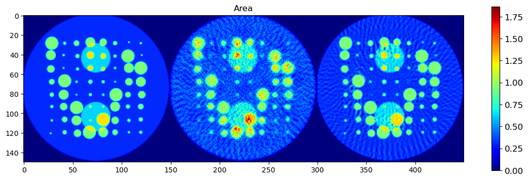
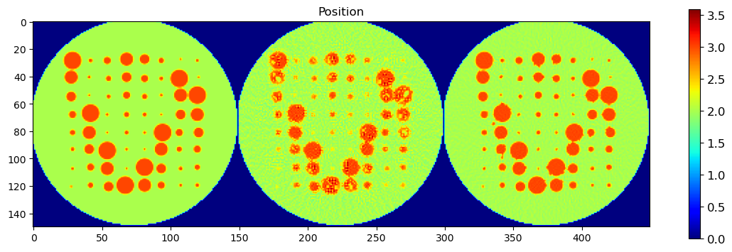
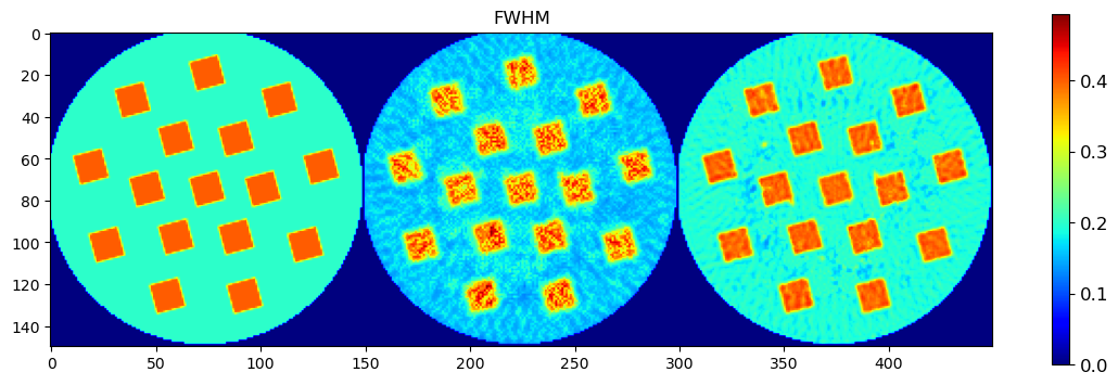
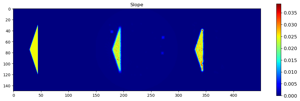
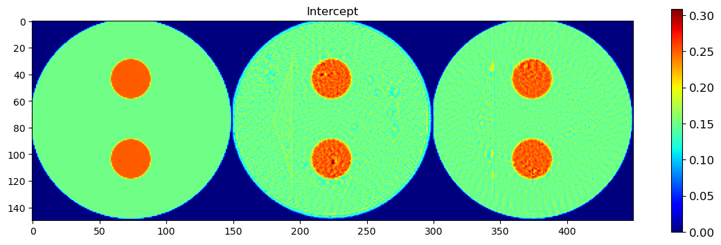
🔍 Patch-Based Sampling on FBP-Reconstructed Volume
This section defines a patch sampling strategy for the FBP + peak fitting pipeline, enabling efficient evaluation or training using the reconstructed volume r as input.
🎯 Purpose
Patch-based sampling allows us to:
Randomly probe local regions of the FBP volume
Enable fair comparison with CNN and DLSR methods that were also trained on patches
Optionally fit peaks or extract local statistics from each patch
🧱 Workflow
Volume and Mask Padding:
Padding is added around the spatial edges of both the FBP volume (
r) and the binary mask.This ensures patches sampled near the boundary are still valid.
Mask Generation:
A binary mask is generated by summing the FBP volume along the spectral axis.
Voxels with non-zero values are marked as valid for sampling.
Patch Index Filtering:
Using
filter_patch_indices(), we identify valid patch locations that overlap with signal.The number of patches per iteration and total number of required iterations to probe the entire image are computed.
Coverage Diagnostic:
A counter tracks how often each voxel is sampled.
This is visualized to ensure spatially uniform coverage across the volume.
📈 Output
The code prints:
Volume and mask shapes after padding
Estimated patch coverage per epoch
Number of required iterations to probe the full image
Number of valid patches available
Visualization of the sampling density
This setup prepares the FBP data for further analysis — for example, comparing peak fitting accuracy or robustness under noisy or undersampled conditions.
[9]:
%matplotlib inline
num_iterations = 100
distribution_type = 'uniform'
std_dev = int(r.shape[0] / 1)
device = 'cuda'
patch_size = 32
num_patches = 16
num_patches_total = 16
mask = np.copy(np.sum(r,axis=2))
mask[mask>0] = 1
mask = np.concatenate((np.zeros((patch_size, mask.shape[1]), dtype='float32'), mask, np.zeros((patch_size, mask.shape[1]), dtype='float32')), axis = 0)
mask = np.concatenate((np.zeros((mask.shape[0], patch_size), dtype='float32'), mask, np.zeros((mask.shape[0], patch_size), dtype='float32')), axis = 1)
volp = np.copy(r)
volp = np.concatenate((np.zeros((patch_size, volp.shape[1], volp.shape[2]), dtype='float32'), volp, np.zeros((patch_size, volp.shape[1], volp.shape[2]), dtype='float32')), axis = 0)
volp = np.concatenate((np.zeros((volp.shape[0], patch_size, volp.shape[2]), dtype='float32'), volp, np.zeros((volp.shape[0], patch_size, volp.shape[2]), dtype='float32')), axis = 1)
rows, cols = volp.shape[0], volp.shape[1] # Size of the matrix
print(volp.shape, r.shape, mask.shape)
plt.figure(1);plt.clf()
plt.imshow(mask)
plt.colorbar()
plt.show()
npix = np.sum(mask)
pcr_probed = 100* (patch_size*patch_size*num_patches)/npix
print(f"Percentage of pixels probed during one epoch: {pcr_probed}")
niters_required = int(np.ceil(100/pcr_probed))
print(f"Number of iterations required to probe full image: {niters_required}")
mask_t = torch.tensor(mask, dtype=torch.bool, device=device)
indices = filter_patch_indices(torch.tensor(mask), patch_size)
print('The number of patches is ', len(indices))
print('The number of iterations (batches) required to probe the whole image is ', int(len(indices)/num_patches) )
counter = initialize_counter(rows, cols)
patch_dimensions = (patch_size, patch_size)
update_counter(counter, indices, patch_dimensions)
print(counter.max())
counter = counter.numpy()
plt.figure(2);plt.clf()
# plt.imshow(counter * mask )
plt.imshow(counter + mask)
# plt.clim(0,1)
plt.colorbar()
plt.show()
print(volp.shape, vol.shape, mask.shape)
(224, 224, 20) (160, 160, 20) (224, 224)
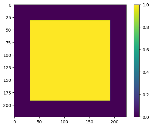
Percentage of pixels probed during one epoch: 64.0
Number of iterations required to probe full image: 2
The number of patches is 25
The number of iterations (batches) required to probe the whole image is 1
tensor(1.)
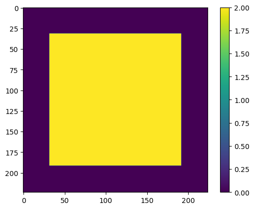
(224, 224, 20) (160, 160, 20) (224, 224)
🔁 Train Parameter Maps on FBP-Reconstructed Volume (FBP + Peak Fitting)
This section trains parameter maps directly on the FBP-reconstructed volume using the same architecture (PrmCNN2D) and training strategy as in the DLSR case. The difference here is that the input data is a reconstructed volume (r) rather than raw sinogram data.
🎯 Purpose
This pipeline simulates the conventional XRD-CT workflow:
Reconstruct the 3D volume using FBP
Fit diffraction patterns voxel-by-voxel to extract physical parameters (area, position, FWHM, etc.)
By training PrmCNN2D to minimize reconstruction error, we obtain spatially smooth parameter maps from the FBP output.
⚙️ Training Configuration
Input:
im_static, a single-channel static image computed from the FBP volumePatch-based training ensures efficiency and robustness
prf = 0.2: enforces stability by soft-clamping parameter predictionsTraining loss is RMSE between the observed FBP voxel spectra and those reconstructed from the fitted parameters
🔁 Training Loop
Each epoch consists of:
Predicting parameter maps (
yc)Clamping predictions and extracting patches
Constructing synthetic spectra from peak + background parameters
Comparing synthetic spectra with the ground truth patches (
yobs)Computing RMSE and updating the model
📈 Output
The model prints:
MAE, MSE, RMSE at intermediate epochs
Accumulated loss over iterations
Total training time and number of completed epochs
This completes the FBP + peak fitting pipeline, enabling direct comparison with DLSR and CNN-based methods in the final evaluation section.
[10]:
npix_x = volp.shape[0]
npix_y = volp.shape[1]
xv = torch.tensor(x, dtype=torch.float32, device='cuda')
### Single peak
peak_definitions = [(1, 1.0, 4.0)]
num_peaks = len(peak_definitions)
num_params_per_peak = 3 # Area, Position, FWHM
background_params = 2 # Slope, Intercept
total_params = num_peaks * num_params_per_peak + background_params
npix = volp.shape[0]
nch_in = total_params
nch_out = total_params
nfilts = 2*total_params # 2*total_params is pretty good when using norm layer
norm_type='layer'
activation='Sigmoid'
downsampling = 8
device = 'cuda'
model = PrmCNN2D(npix, nch_in=nch_in, nch_out=nch_out, nfilts=nfilts, nlayers=1, norm_type='None', prms_layer=True, cnn_layer=False, tensor_vals = 'zeros').to(device)
model_prms = sum(p.numel() for p in model.parameters() if p.requires_grad)
print(f"Total number of parameters: {model_prms}")
print("Conventional number of parameters:", npix*npix*total_params)
def gaussian(x, area, position, fwhm):
"""Gaussian peak shape."""
return area * torch.exp(-(x - position)**2 / (2 * fwhm**2))
MAE = torch.nn.L1Loss()
### Single peak ###
param_min = {
'Area': torch.zeros(num_peaks, dtype=torch.float32).to(device),
'Position': torch.tensor([peak[1] for peak in peak_definitions], dtype=torch.float32).to(device),
'FWHM': torch.zeros(num_peaks, dtype=torch.float32).to(device) + 0.1,
'Fraction': torch.zeros(num_peaks, dtype=torch.float32).to(device),
'Slope': torch.zeros(1, dtype=torch.float32).to(device),
'Intercept': torch.zeros(1, dtype=torch.float32).to(device),
}
param_max = {
'Area': torch.zeros(num_peaks, dtype=torch.float32).to(device) + 2,
'Position': torch.tensor([peak[2] for peak in peak_definitions], dtype=torch.float32).to(device),
'FWHM': torch.zeros(num_peaks, dtype=torch.float32).to(device) + 0.5,
'Fraction': torch.zeros(num_peaks, dtype=torch.float32).to(device) + 1,
'Slope': torch.zeros(1, dtype=torch.float32).to(device) + 0.2,
'Intercept': torch.zeros(1, dtype=torch.float32).to(device) + 0.5,
}
nch = volp.shape[2]
learning_rate = 0.001
epochs = 10000
min_lr = 1E-5
im_static = np.sum(volp, axis=2)
im_static = im_static/np.max(im_static)
im_static = np.reshape(im_static, (1, 1, volp.shape[1], volp.shape[1]))
im_static = torch.tensor(im_static, dtype=torch.float32, device=device)
yobs = np.transpose(volp, (2,1,0))
yobs = torch.tensor(yobs, dtype=torch.float32, device=device)
yobs = torch.reshape(yobs, (1, yobs.shape[0], yobs.shape[1], yobs.shape[2]))
yobs = torch.transpose(yobs, 3, 2)
epochs = 50000
patience = 100 #250
min_lr = 1E-5
learning_rate = 0.1
optimizer = torch.optim.Adam(model.parameters(), lr=learning_rate)
prf = 0.2
scheduler = torch.optim.lr_scheduler.ReduceLROnPlateau(optimizer, patience=patience, factor=0.5, min_lr=min_lr)
num_patches = 16
new_indices = np.array(indices)
total_indices = len(indices)
num_batches = (total_indices + num_patches - 1) // num_patches
print(num_batches)
start = time.time()
logloss = []
for epoch in tqdm(range(epochs)):
loss_acc = 0
for batch_index in range(num_batches):
start_index = batch_index * num_patches
end_index = min(start_index + num_patches, total_indices)
batch_indices = new_indices[start_index:end_index]
yc = model(im_static)
filtered = nn.AvgPool2d(kernel_size=3, stride=1, padding=1)(yc)
lower_bound = filtered * (1 - prf)
upper_bound = filtered * (1 + prf)
yc = torch.clamp(yc, min=lower_bound, max=upper_bound)
yc = calc_patches_indices(batch_indices, yc, patch_size, use_middle=False)
y = torch.zeros((patch_size*patch_size*len(batch_indices), len(xv)), dtype=torch.float32).to(device)
for i in range(num_peaks):
area = denormalize(yc[:, i * 3, :, :], 'Area', param_min, param_max, i)
position = denormalize(yc[:, i * 3 + 1, :, :], 'Position', param_min, param_max, i)
fwhm = denormalize(yc[:, i * 3 + 2, :, :], 'FWHM', param_min, param_max, i)
area = torch.transpose(torch.reshape(area, (area.shape[0], area.shape[1]*area.shape[2])), 1, 0)
position = torch.transpose(torch.reshape(position, (position.shape[0], position.shape[1]*position.shape[2])), 1, 0)
fwhm = torch.transpose(torch.reshape(fwhm, (fwhm.shape[0], fwhm.shape[1]*fwhm.shape[2])), 1, 0)
area = torch.reshape(area, (area.shape[0]*area.shape[1], 1))
position = torch.reshape(position, (area.shape[0]*area.shape[1], 1))
fwhm = torch.reshape(fwhm, (area.shape[0]*area.shape[1], 1))
y += gaussian(xv.unsqueeze(0), area, position, fwhm)
slope = denormalize(yc[:, -2, :, :], 'Slope', param_min, param_max, )
intercept = denormalize(yc[:, -1, :, :], 'Intercept', param_min, param_max, )
slope = torch.transpose(torch.reshape(slope, (slope.shape[0], slope.shape[1]*slope.shape[2])), 1, 0)
intercept = torch.transpose(torch.reshape(intercept, (intercept.shape[0], intercept.shape[1]*intercept.shape[2])), 1, 0)
slope = torch.reshape(slope, (slope.shape[0]*slope.shape[1], 1))
intercept = torch.reshape(intercept, (intercept.shape[0]*intercept.shape[1], 1))
y += slope * xv + intercept
patches = calc_patches_indices(batch_indices, yobs, patch_size, use_middle=False)
patches = torch.reshape(patches, (patches.shape[0],patches.shape[1],patches.shape[2]*patches.shape[3]))
patches = torch.transpose(patches, 1, 2)
patches = torch.transpose(patches, 1, 0)
y = torch.reshape(y, (patches.shape[0], patches.shape[1], nch))
loss_mae = MAE(patches, y)
loss_mse = torch.mean((patches - y) ** 2)
loss_rmse = torch.sqrt(torch.mean((patches - y) ** 2))
loss_acc = loss_acc + loss_rmse
loss = loss_rmse
optimizer.zero_grad()
loss.backward()
optimizer.step()
loss_acc = loss_acc/num_batches
logloss.append(loss_acc.cpu().detach().numpy())
scheduler.step(logloss[-1])
if epoch % (int(patience/2)) == 0:
print('MAE = ', loss_mae, 'MSE = ', loss_mse,'RMSE = ', loss_rmse)
print('Accumulated Loss = ', logloss[-1])
if optimizer.param_groups[0]['lr'] == scheduler.min_lrs[0]:
print("Minimum learning rate reached, stopping the optimization")
print(epoch)
break
total_time = time.time() - start
print(epoch, loss_mae, loss_mse, loss_rmse, logloss[-1])
print(total_time)
Total number of parameters: 250880
Conventional number of parameters: 250880
2
0%| | 7/50000 [00:00<12:47, 65.11it/s]
MAE = tensor(0.4927, device='cuda:0', grad_fn=<MeanBackward0>) MSE = tensor(0.3525, device='cuda:0', grad_fn=<MeanBackward0>) RMSE = tensor(0.5937, device='cuda:0', grad_fn=<SqrtBackward0>)
Accumulated Loss = 0.58584267
0%| | 56/50000 [00:00<12:47, 65.04it/s]
MAE = tensor(0.0321, device='cuda:0', grad_fn=<MeanBackward0>) MSE = tensor(0.0017, device='cuda:0', grad_fn=<MeanBackward0>) RMSE = tensor(0.0416, device='cuda:0', grad_fn=<SqrtBackward0>)
Accumulated Loss = 0.04224749
0%| | 112/50000 [00:01<12:42, 65.41it/s]
MAE = tensor(0.0299, device='cuda:0', grad_fn=<MeanBackward0>) MSE = tensor(0.0015, device='cuda:0', grad_fn=<MeanBackward0>) RMSE = tensor(0.0393, device='cuda:0', grad_fn=<SqrtBackward0>)
Accumulated Loss = 0.03993605
0%| | 161/50000 [00:02<12:21, 67.18it/s]
MAE = tensor(0.0293, device='cuda:0', grad_fn=<MeanBackward0>) MSE = tensor(0.0015, device='cuda:0', grad_fn=<MeanBackward0>) RMSE = tensor(0.0387, device='cuda:0', grad_fn=<SqrtBackward0>)
Accumulated Loss = 0.03938251
0%| | 210/50000 [00:03<12:39, 65.52it/s]
MAE = tensor(0.0291, device='cuda:0', grad_fn=<MeanBackward0>) MSE = tensor(0.0015, device='cuda:0', grad_fn=<MeanBackward0>) RMSE = tensor(0.0384, device='cuda:0', grad_fn=<SqrtBackward0>)
Accumulated Loss = 0.039136857
1%| | 260/50000 [00:03<12:10, 68.05it/s]
MAE = tensor(0.0289, device='cuda:0', grad_fn=<MeanBackward0>) MSE = tensor(0.0015, device='cuda:0', grad_fn=<MeanBackward0>) RMSE = tensor(0.0383, device='cuda:0', grad_fn=<SqrtBackward0>)
Accumulated Loss = 0.039016966
1%| | 309/50000 [00:04<12:32, 66.08it/s]
MAE = tensor(0.0289, device='cuda:0', grad_fn=<MeanBackward0>) MSE = tensor(0.0015, device='cuda:0', grad_fn=<MeanBackward0>) RMSE = tensor(0.0382, device='cuda:0', grad_fn=<SqrtBackward0>)
Accumulated Loss = 0.03892278
1%| | 359/50000 [00:05<12:19, 67.15it/s]
MAE = tensor(0.0288, device='cuda:0', grad_fn=<MeanBackward0>) MSE = tensor(0.0015, device='cuda:0', grad_fn=<MeanBackward0>) RMSE = tensor(0.0382, device='cuda:0', grad_fn=<SqrtBackward0>)
Accumulated Loss = 0.03887009
1%| | 415/50000 [00:06<12:34, 65.74it/s]
MAE = tensor(0.0288, device='cuda:0', grad_fn=<MeanBackward0>) MSE = tensor(0.0015, device='cuda:0', grad_fn=<MeanBackward0>) RMSE = tensor(0.0381, device='cuda:0', grad_fn=<SqrtBackward0>)
Accumulated Loss = 0.038825747
1%| | 457/50000 [00:06<12:30, 66.04it/s]
MAE = tensor(0.0287, device='cuda:0', grad_fn=<MeanBackward0>) MSE = tensor(0.0014, device='cuda:0', grad_fn=<MeanBackward0>) RMSE = tensor(0.0381, device='cuda:0', grad_fn=<SqrtBackward0>)
Accumulated Loss = 0.03879515
1%| | 508/50000 [00:07<12:29, 66.05it/s]
MAE = tensor(0.0287, device='cuda:0', grad_fn=<MeanBackward0>) MSE = tensor(0.0014, device='cuda:0', grad_fn=<MeanBackward0>) RMSE = tensor(0.0381, device='cuda:0', grad_fn=<SqrtBackward0>)
Accumulated Loss = 0.038770676
1%| | 557/50000 [00:08<12:38, 65.19it/s]
MAE = tensor(0.0287, device='cuda:0', grad_fn=<MeanBackward0>) MSE = tensor(0.0014, device='cuda:0', grad_fn=<MeanBackward0>) RMSE = tensor(0.0380, device='cuda:0', grad_fn=<SqrtBackward0>)
Accumulated Loss = 0.038747907
1%| | 613/50000 [00:09<12:36, 65.30it/s]
MAE = tensor(0.0287, device='cuda:0', grad_fn=<MeanBackward0>) MSE = tensor(0.0014, device='cuda:0', grad_fn=<MeanBackward0>) RMSE = tensor(0.0380, device='cuda:0', grad_fn=<SqrtBackward0>)
Accumulated Loss = 0.038733765
1%|▏ | 662/50000 [00:10<12:04, 68.08it/s]
MAE = tensor(0.0286, device='cuda:0', grad_fn=<MeanBackward0>) MSE = tensor(0.0014, device='cuda:0', grad_fn=<MeanBackward0>) RMSE = tensor(0.0380, device='cuda:0', grad_fn=<SqrtBackward0>)
Accumulated Loss = 0.03871785
1%|▏ | 711/50000 [00:10<12:35, 65.25it/s]
MAE = tensor(0.0286, device='cuda:0', grad_fn=<MeanBackward0>) MSE = tensor(0.0014, device='cuda:0', grad_fn=<MeanBackward0>) RMSE = tensor(0.0380, device='cuda:0', grad_fn=<SqrtBackward0>)
Accumulated Loss = 0.03870625
2%|▏ | 760/50000 [00:11<12:30, 65.60it/s]
MAE = tensor(0.0286, device='cuda:0', grad_fn=<MeanBackward0>) MSE = tensor(0.0014, device='cuda:0', grad_fn=<MeanBackward0>) RMSE = tensor(0.0380, device='cuda:0', grad_fn=<SqrtBackward0>)
Accumulated Loss = 0.038691342
2%|▏ | 809/50000 [00:12<12:23, 66.15it/s]
MAE = tensor(0.0286, device='cuda:0', grad_fn=<MeanBackward0>) MSE = tensor(0.0014, device='cuda:0', grad_fn=<MeanBackward0>) RMSE = tensor(0.0380, device='cuda:0', grad_fn=<SqrtBackward0>)
Accumulated Loss = 0.038680073
2%|▏ | 858/50000 [00:12<12:24, 66.01it/s]
MAE = tensor(0.0286, device='cuda:0', grad_fn=<MeanBackward0>) MSE = tensor(0.0014, device='cuda:0', grad_fn=<MeanBackward0>) RMSE = tensor(0.0380, device='cuda:0', grad_fn=<SqrtBackward0>)
Accumulated Loss = 0.038670044
2%|▏ | 907/50000 [00:13<12:27, 65.64it/s]
MAE = tensor(0.0286, device='cuda:0', grad_fn=<MeanBackward0>) MSE = tensor(0.0014, device='cuda:0', grad_fn=<MeanBackward0>) RMSE = tensor(0.0379, device='cuda:0', grad_fn=<SqrtBackward0>)
Accumulated Loss = 0.038662307
2%|▏ | 963/50000 [00:14<12:23, 66.00it/s]
MAE = tensor(0.0286, device='cuda:0', grad_fn=<MeanBackward0>) MSE = tensor(0.0014, device='cuda:0', grad_fn=<MeanBackward0>) RMSE = tensor(0.0379, device='cuda:0', grad_fn=<SqrtBackward0>)
Accumulated Loss = 0.038661756
2%|▏ | 1012/50000 [00:15<12:33, 64.98it/s]
MAE = tensor(0.0286, device='cuda:0', grad_fn=<MeanBackward0>) MSE = tensor(0.0014, device='cuda:0', grad_fn=<MeanBackward0>) RMSE = tensor(0.0379, device='cuda:0', grad_fn=<SqrtBackward0>)
Accumulated Loss = 0.038652554
2%|▏ | 1061/50000 [00:16<12:15, 66.51it/s]
MAE = tensor(0.0286, device='cuda:0', grad_fn=<MeanBackward0>) MSE = tensor(0.0014, device='cuda:0', grad_fn=<MeanBackward0>) RMSE = tensor(0.0379, device='cuda:0', grad_fn=<SqrtBackward0>)
Accumulated Loss = 0.038641036
2%|▏ | 1110/50000 [00:16<12:18, 66.24it/s]
MAE = tensor(0.0286, device='cuda:0', grad_fn=<MeanBackward0>) MSE = tensor(0.0014, device='cuda:0', grad_fn=<MeanBackward0>) RMSE = tensor(0.0379, device='cuda:0', grad_fn=<SqrtBackward0>)
Accumulated Loss = 0.03863822
2%|▏ | 1159/50000 [00:17<12:27, 65.33it/s]
MAE = tensor(0.0286, device='cuda:0', grad_fn=<MeanBackward0>) MSE = tensor(0.0014, device='cuda:0', grad_fn=<MeanBackward0>) RMSE = tensor(0.0379, device='cuda:0', grad_fn=<SqrtBackward0>)
Accumulated Loss = 0.038634375
2%|▏ | 1209/50000 [00:18<12:27, 65.26it/s]
MAE = tensor(0.0286, device='cuda:0', grad_fn=<MeanBackward0>) MSE = tensor(0.0014, device='cuda:0', grad_fn=<MeanBackward0>) RMSE = tensor(0.0379, device='cuda:0', grad_fn=<SqrtBackward0>)
Accumulated Loss = 0.03863038
3%|▎ | 1258/50000 [00:19<12:23, 65.60it/s]
MAE = tensor(0.0285, device='cuda:0', grad_fn=<MeanBackward0>) MSE = tensor(0.0014, device='cuda:0', grad_fn=<MeanBackward0>) RMSE = tensor(0.0379, device='cuda:0', grad_fn=<SqrtBackward0>)
Accumulated Loss = 0.03862448
3%|▎ | 1307/50000 [00:19<12:12, 66.45it/s]
MAE = tensor(0.0286, device='cuda:0', grad_fn=<MeanBackward0>) MSE = tensor(0.0014, device='cuda:0', grad_fn=<MeanBackward0>) RMSE = tensor(0.0379, device='cuda:0', grad_fn=<SqrtBackward0>)
Accumulated Loss = 0.038621664
3%|▎ | 1363/50000 [00:20<12:22, 65.50it/s]
MAE = tensor(0.0286, device='cuda:0', grad_fn=<MeanBackward0>) MSE = tensor(0.0014, device='cuda:0', grad_fn=<MeanBackward0>) RMSE = tensor(0.0379, device='cuda:0', grad_fn=<SqrtBackward0>)
Accumulated Loss = 0.038620017
3%|▎ | 1412/50000 [00:21<12:15, 66.06it/s]
MAE = tensor(0.0285, device='cuda:0', grad_fn=<MeanBackward0>) MSE = tensor(0.0014, device='cuda:0', grad_fn=<MeanBackward0>) RMSE = tensor(0.0379, device='cuda:0', grad_fn=<SqrtBackward0>)
Accumulated Loss = 0.03861794
3%|▎ | 1461/50000 [00:22<12:26, 65.03it/s]
MAE = tensor(0.0285, device='cuda:0', grad_fn=<MeanBackward0>) MSE = tensor(0.0014, device='cuda:0', grad_fn=<MeanBackward0>) RMSE = tensor(0.0379, device='cuda:0', grad_fn=<SqrtBackward0>)
Accumulated Loss = 0.038612567
3%|▎ | 1510/50000 [00:22<12:24, 65.14it/s]
MAE = tensor(0.0285, device='cuda:0', grad_fn=<MeanBackward0>) MSE = tensor(0.0014, device='cuda:0', grad_fn=<MeanBackward0>) RMSE = tensor(0.0379, device='cuda:0', grad_fn=<SqrtBackward0>)
Accumulated Loss = 0.038610715
3%|▎ | 1559/50000 [00:23<12:22, 65.23it/s]
MAE = tensor(0.0285, device='cuda:0', grad_fn=<MeanBackward0>) MSE = tensor(0.0014, device='cuda:0', grad_fn=<MeanBackward0>) RMSE = tensor(0.0379, device='cuda:0', grad_fn=<SqrtBackward0>)
Accumulated Loss = 0.038605884
3%|▎ | 1608/50000 [00:24<12:27, 64.75it/s]
MAE = tensor(0.0285, device='cuda:0', grad_fn=<MeanBackward0>) MSE = tensor(0.0014, device='cuda:0', grad_fn=<MeanBackward0>) RMSE = tensor(0.0379, device='cuda:0', grad_fn=<SqrtBackward0>)
Accumulated Loss = 0.038602117
3%|▎ | 1657/50000 [00:25<12:20, 65.28it/s]
MAE = tensor(0.0285, device='cuda:0', grad_fn=<MeanBackward0>) MSE = tensor(0.0014, device='cuda:0', grad_fn=<MeanBackward0>) RMSE = tensor(0.0378, device='cuda:0', grad_fn=<SqrtBackward0>)
Accumulated Loss = 0.038544387
3%|▎ | 1713/50000 [00:25<12:14, 65.78it/s]
MAE = tensor(0.0285, device='cuda:0', grad_fn=<MeanBackward0>) MSE = tensor(0.0014, device='cuda:0', grad_fn=<MeanBackward0>) RMSE = tensor(0.0378, device='cuda:0', grad_fn=<SqrtBackward0>)
Accumulated Loss = 0.0385435
4%|▎ | 1762/50000 [00:26<12:09, 66.13it/s]
MAE = tensor(0.0285, device='cuda:0', grad_fn=<MeanBackward0>) MSE = tensor(0.0014, device='cuda:0', grad_fn=<MeanBackward0>) RMSE = tensor(0.0378, device='cuda:0', grad_fn=<SqrtBackward0>)
Accumulated Loss = 0.038537346
4%|▎ | 1811/50000 [00:27<12:37, 63.64it/s]
MAE = tensor(0.0285, device='cuda:0', grad_fn=<MeanBackward0>) MSE = tensor(0.0014, device='cuda:0', grad_fn=<MeanBackward0>) RMSE = tensor(0.0378, device='cuda:0', grad_fn=<SqrtBackward0>)
Accumulated Loss = 0.038536653
4%|▎ | 1860/50000 [00:28<12:17, 65.28it/s]
MAE = tensor(0.0285, device='cuda:0', grad_fn=<MeanBackward0>) MSE = tensor(0.0014, device='cuda:0', grad_fn=<MeanBackward0>) RMSE = tensor(0.0378, device='cuda:0', grad_fn=<SqrtBackward0>)
Accumulated Loss = 0.038536362
4%|▍ | 1909/50000 [00:28<12:15, 65.41it/s]
MAE = tensor(0.0285, device='cuda:0', grad_fn=<MeanBackward0>) MSE = tensor(0.0014, device='cuda:0', grad_fn=<MeanBackward0>) RMSE = tensor(0.0378, device='cuda:0', grad_fn=<SqrtBackward0>)
Accumulated Loss = 0.038533393
4%|▍ | 1958/50000 [00:29<12:09, 65.87it/s]
MAE = tensor(0.0285, device='cuda:0', grad_fn=<MeanBackward0>) MSE = tensor(0.0014, device='cuda:0', grad_fn=<MeanBackward0>) RMSE = tensor(0.0378, device='cuda:0', grad_fn=<SqrtBackward0>)
Accumulated Loss = 0.038533177
4%|▍ | 2007/50000 [00:30<12:19, 64.88it/s]
MAE = tensor(0.0285, device='cuda:0', grad_fn=<MeanBackward0>) MSE = tensor(0.0014, device='cuda:0', grad_fn=<MeanBackward0>) RMSE = tensor(0.0378, device='cuda:0', grad_fn=<SqrtBackward0>)
Accumulated Loss = 0.038532883
4%|▍ | 2063/50000 [00:31<12:11, 65.49it/s]
MAE = tensor(0.0285, device='cuda:0', grad_fn=<MeanBackward0>) MSE = tensor(0.0014, device='cuda:0', grad_fn=<MeanBackward0>) RMSE = tensor(0.0378, device='cuda:0', grad_fn=<SqrtBackward0>)
Accumulated Loss = 0.038532134
4%|▍ | 2112/50000 [00:32<12:21, 64.56it/s]
MAE = tensor(0.0285, device='cuda:0', grad_fn=<MeanBackward0>) MSE = tensor(0.0014, device='cuda:0', grad_fn=<MeanBackward0>) RMSE = tensor(0.0378, device='cuda:0', grad_fn=<SqrtBackward0>)
Accumulated Loss = 0.03853111
4%|▍ | 2162/50000 [00:32<11:57, 66.71it/s]
MAE = tensor(0.0285, device='cuda:0', grad_fn=<MeanBackward0>) MSE = tensor(0.0014, device='cuda:0', grad_fn=<MeanBackward0>) RMSE = tensor(0.0378, device='cuda:0', grad_fn=<SqrtBackward0>)
Accumulated Loss = 0.03853079
4%|▍ | 2211/50000 [00:33<12:06, 65.81it/s]
MAE = tensor(0.0285, device='cuda:0', grad_fn=<MeanBackward0>) MSE = tensor(0.0014, device='cuda:0', grad_fn=<MeanBackward0>) RMSE = tensor(0.0378, device='cuda:0', grad_fn=<SqrtBackward0>)
Accumulated Loss = 0.03853023
5%|▍ | 2261/50000 [00:34<11:51, 67.08it/s]
MAE = tensor(0.0285, device='cuda:0', grad_fn=<MeanBackward0>) MSE = tensor(0.0014, device='cuda:0', grad_fn=<MeanBackward0>) RMSE = tensor(0.0378, device='cuda:0', grad_fn=<SqrtBackward0>)
Accumulated Loss = 0.038530104
5%|▍ | 2310/50000 [00:35<12:07, 65.56it/s]
MAE = tensor(0.0285, device='cuda:0', grad_fn=<MeanBackward0>) MSE = tensor(0.0014, device='cuda:0', grad_fn=<MeanBackward0>) RMSE = tensor(0.0378, device='cuda:0', grad_fn=<SqrtBackward0>)
Accumulated Loss = 0.038529754
5%|▍ | 2359/50000 [00:35<12:13, 64.92it/s]
MAE = tensor(0.0285, device='cuda:0', grad_fn=<MeanBackward0>) MSE = tensor(0.0014, device='cuda:0', grad_fn=<MeanBackward0>) RMSE = tensor(0.0378, device='cuda:0', grad_fn=<SqrtBackward0>)
Accumulated Loss = 0.03852971
5%|▍ | 2408/50000 [00:36<12:05, 65.63it/s]
MAE = tensor(0.0285, device='cuda:0', grad_fn=<MeanBackward0>) MSE = tensor(0.0014, device='cuda:0', grad_fn=<MeanBackward0>) RMSE = tensor(0.0378, device='cuda:0', grad_fn=<SqrtBackward0>)
Accumulated Loss = 0.038529508
5%|▍ | 2457/50000 [00:37<12:02, 65.79it/s]
MAE = tensor(0.0285, device='cuda:0', grad_fn=<MeanBackward0>) MSE = tensor(0.0014, device='cuda:0', grad_fn=<MeanBackward0>) RMSE = tensor(0.0378, device='cuda:0', grad_fn=<SqrtBackward0>)
Accumulated Loss = 0.038529485
5%|▌ | 2513/50000 [00:38<12:00, 65.90it/s]
MAE = tensor(0.0285, device='cuda:0', grad_fn=<MeanBackward0>) MSE = tensor(0.0014, device='cuda:0', grad_fn=<MeanBackward0>) RMSE = tensor(0.0378, device='cuda:0', grad_fn=<SqrtBackward0>)
Accumulated Loss = 0.03852939
5%|▌ | 2562/50000 [00:38<12:06, 65.32it/s]
MAE = tensor(0.0285, device='cuda:0', grad_fn=<MeanBackward0>) MSE = tensor(0.0014, device='cuda:0', grad_fn=<MeanBackward0>) RMSE = tensor(0.0378, device='cuda:0', grad_fn=<SqrtBackward0>)
Accumulated Loss = 0.03852937
5%|▌ | 2611/50000 [00:39<12:02, 65.60it/s]
MAE = tensor(0.0285, device='cuda:0', grad_fn=<MeanBackward0>) MSE = tensor(0.0014, device='cuda:0', grad_fn=<MeanBackward0>) RMSE = tensor(0.0378, device='cuda:0', grad_fn=<SqrtBackward0>)
Accumulated Loss = 0.038529318
5%|▌ | 2660/50000 [00:40<11:53, 66.35it/s]
MAE = tensor(0.0285, device='cuda:0', grad_fn=<MeanBackward0>) MSE = tensor(0.0014, device='cuda:0', grad_fn=<MeanBackward0>) RMSE = tensor(0.0378, device='cuda:0', grad_fn=<SqrtBackward0>)
Accumulated Loss = 0.038529314
5%|▌ | 2709/50000 [00:41<12:01, 65.53it/s]
MAE = tensor(0.0285, device='cuda:0', grad_fn=<MeanBackward0>) MSE = tensor(0.0014, device='cuda:0', grad_fn=<MeanBackward0>) RMSE = tensor(0.0378, device='cuda:0', grad_fn=<SqrtBackward0>)
Accumulated Loss = 0.038529284
6%|▌ | 2758/50000 [00:41<11:58, 65.80it/s]
MAE = tensor(0.0285, device='cuda:0', grad_fn=<MeanBackward0>) MSE = tensor(0.0014, device='cuda:0', grad_fn=<MeanBackward0>) RMSE = tensor(0.0378, device='cuda:0', grad_fn=<SqrtBackward0>)
Accumulated Loss = 0.038529277
6%|▌ | 2814/50000 [00:42<12:09, 64.65it/s]
MAE = tensor(0.0285, device='cuda:0', grad_fn=<MeanBackward0>) MSE = tensor(0.0014, device='cuda:0', grad_fn=<MeanBackward0>) RMSE = tensor(0.0378, device='cuda:0', grad_fn=<SqrtBackward0>)
Accumulated Loss = 0.038529277
6%|▌ | 2863/50000 [00:43<11:58, 65.58it/s]
MAE = tensor(0.0285, device='cuda:0', grad_fn=<MeanBackward0>) MSE = tensor(0.0014, device='cuda:0', grad_fn=<MeanBackward0>) RMSE = tensor(0.0378, device='cuda:0', grad_fn=<SqrtBackward0>)
Accumulated Loss = 0.038529262
6%|▌ | 2912/50000 [00:44<12:01, 65.23it/s]
MAE = tensor(0.0285, device='cuda:0', grad_fn=<MeanBackward0>) MSE = tensor(0.0014, device='cuda:0', grad_fn=<MeanBackward0>) RMSE = tensor(0.0378, device='cuda:0', grad_fn=<SqrtBackward0>)
Accumulated Loss = 0.038529262
6%|▌ | 2961/50000 [00:44<12:08, 64.60it/s]
MAE = tensor(0.0285, device='cuda:0', grad_fn=<MeanBackward0>) MSE = tensor(0.0014, device='cuda:0', grad_fn=<MeanBackward0>) RMSE = tensor(0.0378, device='cuda:0', grad_fn=<SqrtBackward0>)
Accumulated Loss = 0.038529254
6%|▌ | 3010/50000 [00:45<12:00, 65.19it/s]
MAE = tensor(0.0285, device='cuda:0', grad_fn=<MeanBackward0>) MSE = tensor(0.0014, device='cuda:0', grad_fn=<MeanBackward0>) RMSE = tensor(0.0378, device='cuda:0', grad_fn=<SqrtBackward0>)
Accumulated Loss = 0.038529247
6%|▌ | 3059/50000 [00:46<11:51, 66.02it/s]
MAE = tensor(0.0285, device='cuda:0', grad_fn=<MeanBackward0>) MSE = tensor(0.0014, device='cuda:0', grad_fn=<MeanBackward0>) RMSE = tensor(0.0378, device='cuda:0', grad_fn=<SqrtBackward0>)
Accumulated Loss = 0.038529247
6%|▌ | 3108/50000 [00:47<11:51, 65.89it/s]
MAE = tensor(0.0285, device='cuda:0', grad_fn=<MeanBackward0>) MSE = tensor(0.0014, device='cuda:0', grad_fn=<MeanBackward0>) RMSE = tensor(0.0378, device='cuda:0', grad_fn=<SqrtBackward0>)
Accumulated Loss = 0.038529247
6%|▋ | 3135/50000 [00:47<11:52, 65.82it/s]
Minimum learning rate reached, stopping the optimization
3135
3135 tensor(0.0285, device='cuda:0', grad_fn=<MeanBackward0>) tensor(0.0014, device='cuda:0', grad_fn=<MeanBackward0>) tensor(0.0378, device='cuda:0', grad_fn=<SqrtBackward0>) 0.038529247
47.649693727493286
🖼️ Visualize FBP + Peak Fitting Parameter Maps vs. Ground Truth
We now extract and visualize the parameter maps obtained by fitting the FBP-reconstructed volume using the PrmCNN2D model. This completes our comparison of the three reconstruction strategies:
Ground Truth
DLSR-prm
DLSR-PeakFitCNN
FBP + Peak Fitting
🧱 Post-Processing
A final forward pass is used to extract the fitted parameters from the trained FBP-based model.
Maps are locally smoothed and clamped for stability.
Parameters are then denormalized into physical units.
The resulting maps are cropped to match the ground truth shape and masked using the same binary mask (msk) to ignore background regions.
🗺️ Comparison Layout
For each parameter:
We concatenate two maps side-by-side:
Left: Ground truth
Right: FBP + fitted parameter map (masked)
This is done for:
Peak Area
Peak Position
Peak FWHM
Background Slope
Background Intercept
These plots allow direct qualitative comparison with the maps generated via DLSR and PeakFitCNN, helping identify artefacts, smoothness, and fidelity under undersampled conditions.
[40]:
%matplotlib inline
ims = model(im_static)
filtered = nn.AvgPool2d(kernel_size=5, stride=1, padding=2)(ims)
lower_bound = filtered * (1 - prf)
upper_bound = filtered * (1 + prf)
ims = torch.clamp(ims, min=lower_bound, max=upper_bound)
i = 0
prms_peak1_area = denormalize(ims[:, i * 3, :, :], 'Area', param_min, param_max, i)[0,:,:].cpu().detach().numpy()
prms_peak1_pos = denormalize(ims[:, i * 3 + 1, :, :], 'Position', param_min, param_max, i)[0,:,:].cpu().detach().numpy()
prms_peak1_fwhm = denormalize(ims[:, i * 3 + 2, :, :], 'FWHM', param_min, param_max, i)[0,:,:].cpu().detach().numpy()
prms_slope = denormalize(ims[:, -2, :, :], 'Slope', param_min, param_max, )[0,:,:].cpu().detach().numpy()
prms_intercept = denormalize(ims[:, -1, :, :], 'Intercept', param_min, param_max, )[0,:,:].cpu().detach().numpy()
ofs = int((prms_peak1_area.shape[0] - peak_area.shape[0])/2)
prms_peak1_area = prms_peak1_area[ofs:prms_peak1_area.shape[0]-ofs, ofs:prms_peak1_area.shape[1]-ofs]
prms_peak1_pos = prms_peak1_pos[ofs:prms_peak1_pos.shape[0]-ofs, ofs:prms_peak1_pos.shape[1]-ofs]
prms_peak1_fwhm = prms_peak1_fwhm[ofs:prms_peak1_fwhm.shape[0]-ofs, ofs:prms_peak1_fwhm.shape[1]-ofs]
prms_slope = prms_slope[ofs:prms_slope.shape[0]-ofs, ofs:prms_slope.shape[1]-ofs]
prms_intercept = prms_intercept[ofs:prms_intercept.shape[0]-ofs, ofs:prms_intercept.shape[1]-ofs]
msk = np.copy(peak_area)
msk[msk<0.1] = 0
msk[msk>0] = 1
areac = np.concatenate((peak_area, np.transpose(prms_peak1_area*msk)), axis = 1)
posc = np.concatenate((peak_position, np.transpose(prms_peak1_pos*msk)), axis = 1)
fwhmc = np.concatenate((peak_fwhm, np.transpose(prms_peak1_fwhm*msk)), axis = 1)
slopec = np.concatenate((peak_slope, np.transpose(prms_slope*msk)), axis = 1)
interceptc = np.concatenate((peak_intercept, np.transpose(prms_intercept*msk)), axis = 1)
plt.figure(1, figsize=(14,14));plt.clf()
h = plt.imshow(areac)
cbar = plt.colorbar(h, shrink=0.4)
cbar.ax.tick_params(labelsize=12)
plt.title('Area')
plt.show()
plt.figure(2, figsize=(14,14));plt.clf()
h = plt.imshow(posc)
cbar = plt.colorbar(h, shrink=0.4)
cbar.ax.tick_params(labelsize=12)
plt.title('Position')
plt.show()
plt.figure(3, figsize=(14,14));plt.clf()
h = plt.imshow(fwhmc)
cbar = plt.colorbar(h, shrink=0.4)
cbar.ax.tick_params(labelsize=12)
plt.title('FWHM')
plt.show()
plt.figure(4, figsize=(14,14));plt.clf()
h = plt.imshow(slopec)
cbar = plt.colorbar(h, shrink=0.4)
cbar.ax.tick_params(labelsize=12)
plt.title('Slope')
plt.show()
plt.figure(5, figsize=(14,14));plt.clf()
h = plt.imshow(interceptc)
cbar = plt.colorbar(h, shrink=0.4)
cbar.ax.tick_params(labelsize=12)
plt.title('Intercept')
plt.show()
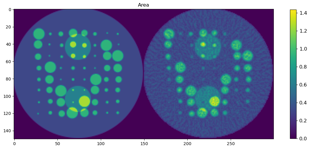
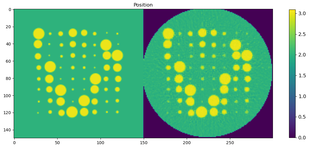
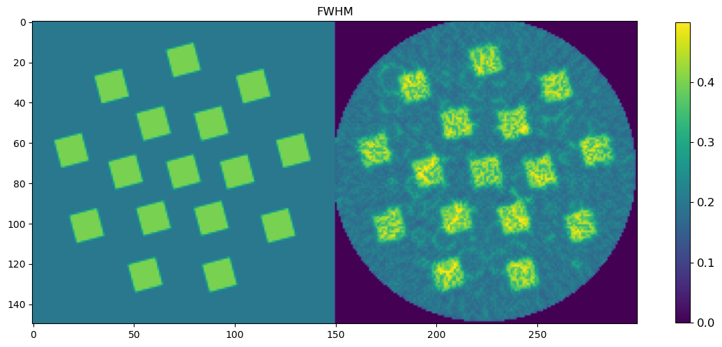
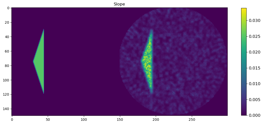
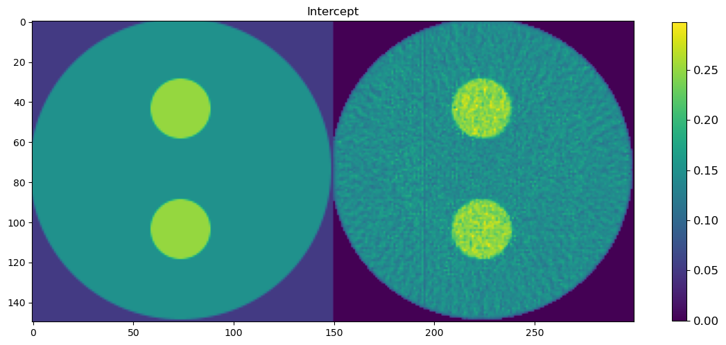
🧪 Final Comparison: Ground Truth vs FBP-Fit vs DLSR-prm vs DLSR-PeakFitCNN
We now present a unified side-by-side visual comparison of the parameter maps produced by:
Ground Truth — from the original synthetic phantom
FBP + Peak Fitting — fitted using
PrmCNN2Don the FBP-reconstructed volumeDLSR-prm — fitted using
PrmCNN2Dusing the DLSR approach with the sinogram dataDLSR-PeakFitCNN — directly predicted from 4× downsampled input using a self-supervised CNN
📌 Parameters Compared
Peak Area
Peak Position
Peak FWHM
Background Slope
Background Intercept
Each subplot displays the four maps concatenated horizontally:
First: Ground truth
Seconnd: FBP + peak fit
Third: DLSR-prm
Fourth: DLSR-PeakFitCNN
🔍 Purpose
This visualization enables direct assessment of:
Spatial fidelity: How well each method recovers sharp features and gradients
Noise resilience: Suppression of artefacts, especially in low-signal regions
Biases or smoothing effects from CNN regularization or FBP artefacts
By comparing all approaches under the same visualization layout, we can appreciate the strengths and weaknesses of each pipeline.
In the next and final section, we’ll summarize key findings and reflect on implications for real-world XRD-CT analysis and future directions.
[45]:
%matplotlib inline
ims = model_cnn(downsampled)
filtered = nn.AvgPool2d(kernel_size=3, stride=1, padding=1)(ims)
lower_bound = filtered * (1 - prf)
upper_bound = filtered * (1 + prf)
ims = torch.clamp(ims, min=lower_bound, max=upper_bound)
i = 0
cnn_peak1_area = denormalize(ims[:, i * 3, :, :], 'Area', param_min, param_max, i)[0,:,:].cpu().detach().numpy()
cnn_peak1_pos = denormalize(ims[:, i * 3 + 1, :, :], 'Position', param_min, param_max, i)[0,:,:].cpu().detach().numpy()
cnn_peak1_fwhm = denormalize(ims[:, i * 3 + 2, :, :], 'FWHM', param_min, param_max, i)[0,:,:].cpu().detach().numpy()
cnn_slope = denormalize(ims[:, -2, :, :], 'Slope', param_min, param_max, )[0,:,:].cpu().detach().numpy()
cnn_intercept = denormalize(ims[:, -1, :, :], 'Intercept', param_min, param_max, )[0,:,:].cpu().detach().numpy()
ofs = int((cnn_peak1_area.shape[0] - peak_area.shape[0])/2)
cnn_peak1_area = cnn_peak1_area[ofs:cnn_peak1_area.shape[0]-ofs, ofs:cnn_peak1_area.shape[1]-ofs]
cnn_peak1_pos = cnn_peak1_pos[ofs:cnn_peak1_pos.shape[0]-ofs, ofs:cnn_peak1_pos.shape[1]-ofs]
cnn_peak1_fwhm = cnn_peak1_fwhm[ofs:cnn_peak1_fwhm.shape[0]-ofs, ofs:cnn_peak1_fwhm.shape[1]-ofs]
cnn_slope = cnn_slope[ofs:cnn_slope.shape[0]-ofs, ofs:cnn_slope.shape[1]-ofs]
cnn_intercept = cnn_intercept[ofs:cnn_intercept.shape[0]-ofs, ofs:cnn_intercept.shape[1]-ofs]
msk = np.copy(peak_area)
msk[msk<0.1] = 0
msk[msk>0] = 1
areac = np.concatenate((peak_area*msk, np.transpose(prms_peak1_area)*msk, prms_peak1_area_dlsr*msk, cnn_peak1_area*msk), axis = 1)
posc = np.concatenate((peak_position*msk, np.transpose(prms_peak1_pos)*msk, prms_peak1_pos_dlsr*msk,cnn_peak1_pos*msk), axis = 1)
fwhmc = np.concatenate((peak_fwhm*msk, np.transpose(prms_peak1_fwhm)*msk, prms_peak1_fwhm_dlsr*msk,cnn_peak1_fwhm*msk), axis = 1)
slopec = np.concatenate((peak_slope*msk, np.transpose(prms_slope)*msk, prms_slope_dlsr*msk,cnn_slope*msk), axis = 1)
interceptc = np.concatenate((peak_intercept*msk, np.transpose(prms_intercept)*msk, prms_intercept_dlsr*msk,cnn_intercept*msk), axis = 1)
plt.figure(1, figsize=(20,20));plt.clf()
h = plt.imshow(areac, cmap = 'jet')
cbar = plt.colorbar(h, shrink=0.25)
cbar.ax.tick_params(labelsize=12)
plt.title('Area')
plt.show()
plt.figure(2, figsize=(20,20));plt.clf()
h = plt.imshow(posc, cmap = 'jet')
cbar = plt.colorbar(h, shrink=0.25)
cbar.ax.tick_params(labelsize=12)
plt.title('Position')
plt.show()
plt.figure(3, figsize=(20,20));plt.clf()
h = plt.imshow(fwhmc, cmap = 'jet')
cbar = plt.colorbar(h, shrink=0.25)
cbar.ax.tick_params(labelsize=12)
plt.title('FWHM')
plt.show()
plt.figure(4, figsize=(20,20));plt.clf()
h = plt.imshow(slopec, cmap = 'jet')
cbar = plt.colorbar(h, shrink=0.25)
cbar.ax.tick_params(labelsize=12)
plt.title('Slope')
plt.show()
plt.figure(5, figsize=(20,20));plt.clf()
h = plt.imshow(interceptc, cmap = 'jet')
cbar = plt.colorbar(h, shrink=0.25)
cbar.ax.tick_params(labelsize=12)
plt.title('Intercept')
plt.show()
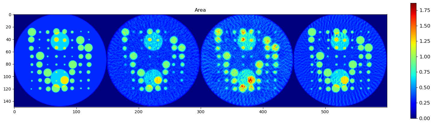
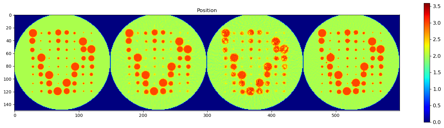
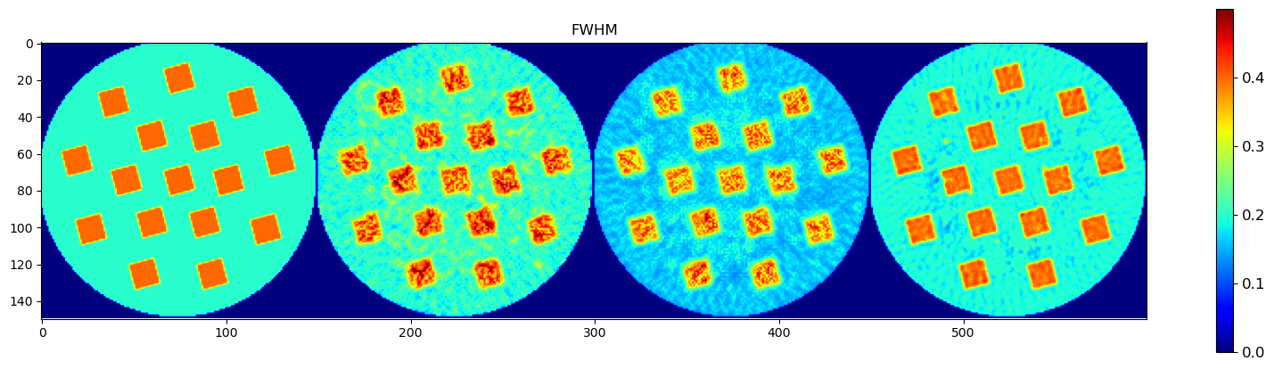
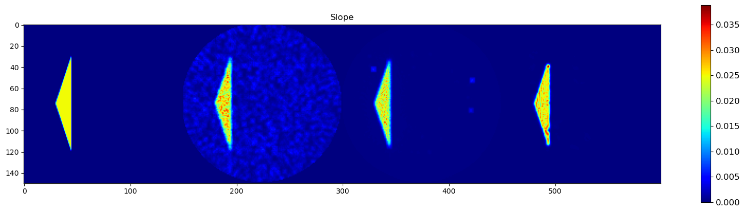
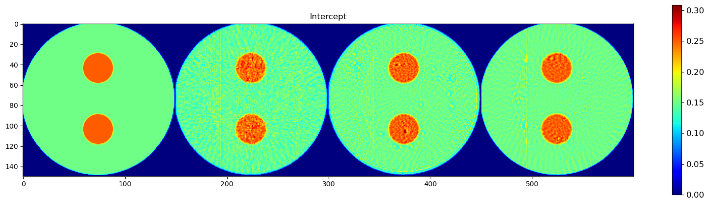
💾 Save Processed Parameter Maps to HDF5
To facilitate downstream analysis and reproducibility, we save all relevant parameter maps to an HDF5 file (dlsr_results.h5). This includes:
Ground truth maps (
*_gt) from the synthetic simulationDLSR-PeakFitCNN predictions (
*_dlsr_cnn) obtained fromPeakFitCNNDLSR-prm predictions (
*_dlsr_prms) obtained fromPrmCNN2DFBP-prm predictions (
*_fbp_prms) obtained fromPrmCNN2DSide-by-side concatenated maps (
*_concat) used for visualization
All maps are masked (msk) to include only signal-rich regions. The file is stored in the examples/results/ directory of the nDTomo package using a relative path resolved by ndtomopath().
This step ensures a compact, structured format for easy sharing, reproducibility, and integration with other analysis or visualization tools.
[46]:
import h5py, os
from nDTomo.methods.misc import ndtomopath
fn = os.path.join(ndtomopath(), 'examples', 'results', 'dlsr_results.h5')
with h5py.File(fn, 'w') as f:
f.create_dataset('peak_area_gt', data=peak_area*msk)
f.create_dataset('peak_area_dlsr_cnn', data=cnn_peak1_area*msk)
f.create_dataset('peak_area_dlsr_prms', data=prms_peak1_area_dlsr*msk)
f.create_dataset('peak_area_fbp_prms', data=prms_peak1_area*msk)
f.create_dataset('peak_position_gt', data=peak_position*msk)
f.create_dataset('peak_position_dlsr_cnn', data=cnn_peak1_pos*msk)
f.create_dataset('peak_position_dlsr_prms', data=prms_peak1_pos_dlsr*msk)
f.create_dataset('peak_position_fbp_prms', data=prms_peak1_pos*msk)
f.create_dataset('peak_fwhm_gt', data=peak_fwhm*msk)
f.create_dataset('peak_fwhm_dlsr_cnn', data=cnn_peak1_fwhm*msk)
f.create_dataset('peak_fwhm_dlsr_prms', data=prms_peak1_fwhm_dlsr*msk)
f.create_dataset('peak_fwhm_fbp_prms', data=prms_peak1_fwhm*msk)
f.create_dataset('peak_slope_gt', data=peak_slope*msk)
f.create_dataset('peak_slope_dlsr_cnn', data=cnn_slope*msk)
f.create_dataset('peak_slope_dlsr_prms', data=prms_slope_dlsr*msk)
f.create_dataset('peak_slope_fbp_prms', data=prms_slope*msk)
f.create_dataset('peak_intercept_gt', data=peak_intercept*msk)
f.create_dataset('peak_intercept_dlsr_cnn', data=cnn_intercept*msk)
f.create_dataset('peak_intercept_dlsr_prms', data=prms_intercept_dlsr*msk)
f.create_dataset('peak_intercept_fbp_prms', data=prms_intercept*msk)
f.create_dataset('peak_area_concat', data=areac)
f.create_dataset('peak_position_concat', data=posc)
f.create_dataset('peak_fwhm_concat', data=fwhmc)
f.create_dataset('peak_slope_concat', data=slopec)
f.create_dataset('peak_intercept_concat', data=interceptc)
📏 Define Evaluation Metrics
To quantitatively compare the CNN-predicted and conventionally fitted parameter maps against the ground truth, we implement the following standard image quality metrics using NumPy and scikit-image:
- MAE (Mean Absolute Error):Measures the average absolute difference between the predicted and ground truth values.
- MSE (Mean Squared Error):Measures the average of the squared differences, penalizing larger errors more heavily.
- RMSE (Root Mean Squared Error):The square root of MSE. While MSE penalizes larger errors more heavily due to squaring, RMSE transforms the result back to the original data scale, making it easier to interpret. It retains the sensitivity to large errors but is more directly comparable to the magnitude of the target values.
- PSNR (Peak Signal-to-Noise Ratio):Indicates the ratio between the maximum possible signal and the noise introduced by prediction errors. Higher values imply better fidelity.
SSIM (Structural Similarity Index): Evaluates perceived quality by comparing local patterns of pixel intensities. It accounts for luminance, contrast, and structural differences.
[78]:
import numpy as np
from skimage.metrics import structural_similarity as ssim_skimage
def mae(gt, pred):
return np.mean(np.abs(gt - pred))
def mse(gt, pred):
return np.mean((gt - pred)**2)
def rmse(gt, pred):
return np.sqrt(mse(gt, pred))
def psnr(gt, pred, data_range=None):
if data_range is None:
data_range = gt.max() - gt.min()
return 20 * np.log10(data_range) - 10 * np.log10(mse(gt, pred))
def ssim(gt, pred, data_range=None):
if data_range is None:
data_range = gt.max() - gt.min()
return ssim_skimage(gt, pred, data_range=data_range)
def plot_results(gt, cnn, prms_dlsr, prms, label, folder=None):
if folder is None:
folder = os.path.join(ndtomopath(), 'examples', 'results')
mae_vals = [
mae(gt, cnn),
mae(gt, prms_dlsr),
mae(gt, prms)
]
ssim_vals = [
ssim(gt, cnn),
ssim(gt, prms_dlsr),
ssim(gt, prms)
]
mse_vals = [
mse(gt, cnn),
mse(gt, prms_dlsr),
mse(gt, prms)
]
rmse_vals = [
rmse(gt, cnn),
rmse(gt, prms_dlsr),
rmse(gt, prms)
]
psnr_vals = [
psnr(gt, cnn),
psnr(gt, prms_dlsr),
psnr(gt, prms)
]
# Labels
methods = ['DLSR-PeakFitCNN', 'DLSR-prms', 'FBP-prms']
metrics = ['MAE', 'SSIM', 'MSE', 'RMSE', 'PSNR']
all_metrics = [mae_vals, ssim_vals, mse_vals, rmse_vals, psnr_vals]
# Plot each metric in a separate figure
for i, (metric_name, values) in enumerate(zip(metrics, all_metrics)):
plt.figure(figsize=(6, 5))
bars = plt.bar(methods, values)
# Annotate bars with values
for bar in bars:
height = bar.get_height()
plt.text(bar.get_x() + bar.get_width()/2, height * 1.01, f'{height:.6f}',
ha='center', va='bottom', fontsize=10)
plt.ylabel(metric_name)
plt.title(f'{label} {metric_name} Comparison')
plt.grid(axis='y', linestyle='--', alpha=0.6)
plt.tight_layout()
plt.savefig(os.path.join(folder, f'{label}_{metric_name}_dlsr.png'), dpi=300)
plt.show()
[79]:
gt = peak_area * msk
cnn = cnn_peak1_area * msk
prms_dlsr = prms_peak1_area_dlsr * msk
prms = prms_peak1_area * msk
print("CNN MAE:", mae(gt, cnn))
print("PRMS DLSR MAE:", mae(gt, prms_dlsr))
print("PRMS MAE:", mae(gt, prms))
print('----------')
print("CNN SSIM:", ssim(gt, cnn))
print("PRMS DLSR SSIM:", ssim(gt, prms_dlsr))
print("PRMS SSIM:", ssim(gt, prms))
print('----------')
print("CNN MSE:", mse(gt, cnn))
print("PRMS DLSR MSE:", mse(gt, prms_dlsr))
print("PRMS MSE:", mse(gt, prms))
print('----------')
print("CNN RMSE:", rmse(gt, cnn))
print("PRMS DLSR RMSE:", rmse(gt, prms_dlsr))
print("PRMS RMSE:", rmse(gt, prms))
print('----------')
print("CNN PSNR:", psnr(gt, cnn))
print("PRMS DLSR PSNR:", psnr(gt, prms_dlsr))
print("PRMS PSNR:", psnr(gt, prms))
plot_results(gt, cnn, prms_dlsr, prms, label='Area')
CNN MAE: 0.032880998292062515
PRMS DLSR MAE: 0.07094472231544013
PRMS MAE: 0.10637854429075828
----------
CNN SSIM: 0.7631768138539838
PRMS DLSR SSIM: 0.5974951999440254
PRMS SSIM: 0.47537739079722724
----------
CNN MSE: 0.0025517945926493246
PRMS DLSR MSE: 0.011779700975874498
PRMS MSE: 0.04090083879385902
----------
CNN RMSE: 0.05051529068162752
PRMS DLSR RMSE: 0.10853433086297855
PRMS RMSE: 0.20223955793528384
----------
CNN PSNR: 27.869743132041453
PRMS DLSR PSNR: 21.22685759858403
PRMS PSNR: 15.82087811411973
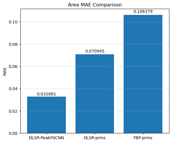
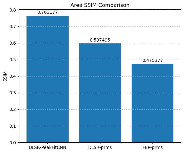
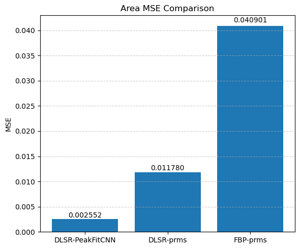
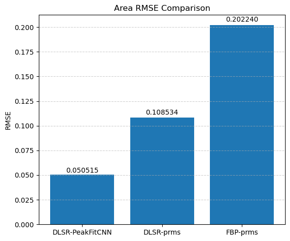
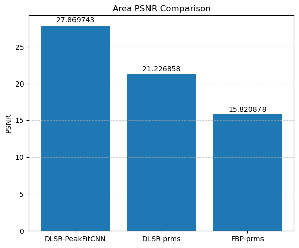
[80]:
gt = peak_position * msk
cnn = cnn_peak1_pos * msk
prms_dlsr = prms_peak1_pos_dlsr * msk
prms = prms_peak1_pos * msk
print("CNN MAE:", mae(gt, cnn))
print("PRMS DLSR MAE:", mae(gt, prms_dlsr))
print("PRMS MAE:", mae(gt, prms))
print('----------')
print("CNN SSIM:", ssim(gt, cnn))
print("PRMS DLSR SSIM:", ssim(gt, prms_dlsr))
print("PRMS SSIM:", ssim(gt, prms))
print('----------')
print("CNN MSE:", mse(gt, cnn))
print("PRMS DLSR MSE:", mse(gt, prms_dlsr))
print("PRMS MSE:", mse(gt, prms))
print('----------')
print("CNN RMSE:", rmse(gt, cnn))
print("PRMS DLSR RMSE:", rmse(gt, prms_dlsr))
print("PRMS RMSE:", rmse(gt, prms))
print('----------')
print("CNN PSNR:", psnr(gt, cnn))
print("PRMS DLSR PSNR:", psnr(gt, prms_dlsr))
print("PRMS PSNR:", psnr(gt, prms))
plot_results(gt, cnn, prms_dlsr, prms, label='Position')
CNN MAE: 0.037078241829813265
PRMS DLSR MAE: 0.09985590337627709
PRMS MAE: 0.13296028588554007
----------
CNN SSIM: 0.880240597746252
PRMS DLSR SSIM: 0.6534935643442704
PRMS SSIM: 0.6355206333235536
----------
CNN MSE: 0.004254889381996164
PRMS DLSR MSE: 0.025488439627958902
PRMS MSE: 0.09089050909190784
----------
CNN RMSE: 0.06522951312094982
PRMS DLSR RMSE: 0.1596509931944017
PRMS RMSE: 0.30148052854522434
----------
CNN PSNR: 33.253542355975995
PRMS DLSR PSNR: 25.478992601493253
PRMS PSNR: 19.95723973458388
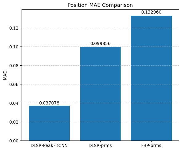
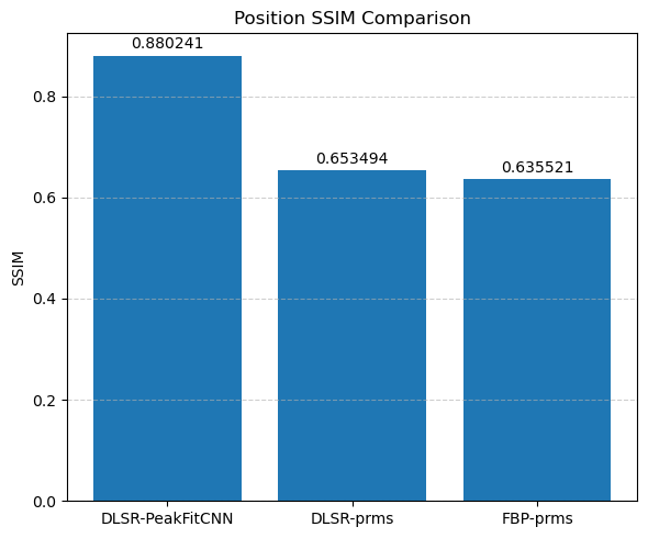
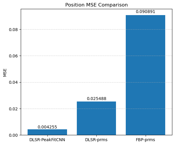
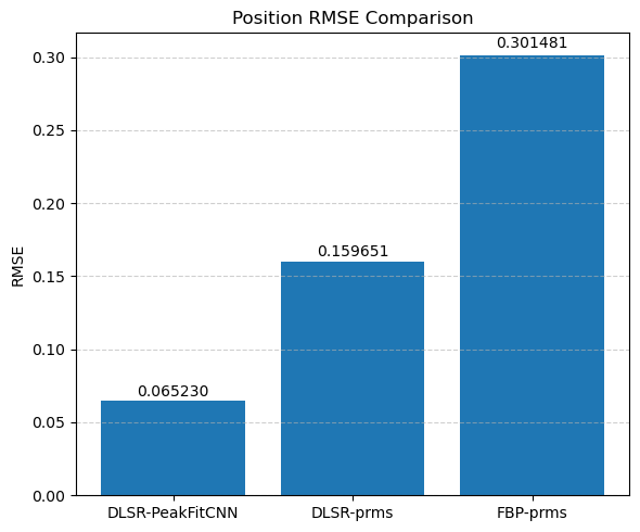
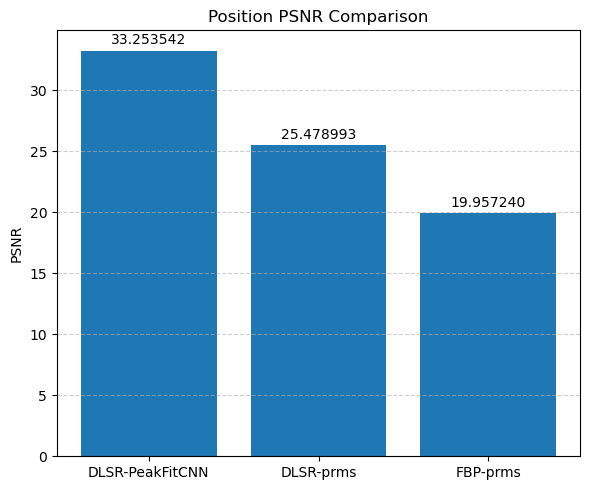
[81]:
gt = peak_fwhm * msk
cnn = cnn_peak1_fwhm * msk
prms_dlsr = prms_peak1_fwhm_dlsr * msk
prms = prms_peak1_fwhm * msk
print("CNN MAE:", mae(gt, cnn))
print("PRMS DLSR MAE:", mae(gt, prms_dlsr))
print("PRMS MAE:", mae(gt, prms))
print('----------')
print("CNN SSIM:", ssim(gt, cnn))
print("PRMS DLSR SSIM:", ssim(gt, prms_dlsr))
print("PRMS SSIM:", ssim(gt, prms))
print('----------')
print("CNN MSE:", mse(gt, cnn))
print("PRMS DLSR MSE:", mse(gt, prms_dlsr))
print("PRMS MSE:", mse(gt, prms))
print('----------')
print("CNN RMSE:", rmse(gt, cnn))
print("PRMS DLSR RMSE:", rmse(gt, prms_dlsr))
print("PRMS RMSE:", rmse(gt, prms))
print('----------')
print("CNN PSNR:", psnr(gt, cnn))
print("PRMS DLSR PSNR:", psnr(gt, prms_dlsr))
print("PRMS PSNR:", psnr(gt, prms))
plot_results(gt, cnn, prms_dlsr, prms, label='FWHM')
CNN MAE: 0.009734031967542793
PRMS DLSR MAE: 0.029672065857338975
PRMS MAE: 0.05247869552229657
----------
CNN SSIM: 0.7873608882599813
PRMS DLSR SSIM: 0.6535973294229542
PRMS SSIM: 0.3131377568093183
----------
CNN MSE: 0.00021778565586626588
PRMS DLSR MSE: 0.0014917452992159756
PRMS MSE: 0.008195099691559663
----------
CNN RMSE: 0.014757562666858843
PRMS DLSR RMSE: 0.038623118714262
PRMS RMSE: 0.09052678991083062
----------
CNN PSNR: 28.660907104651628
PRMS DLSR PSNR: 20.30425304685309
PRMS PSNR: 12.905657416217792
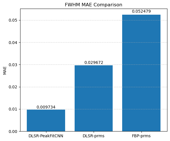
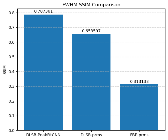
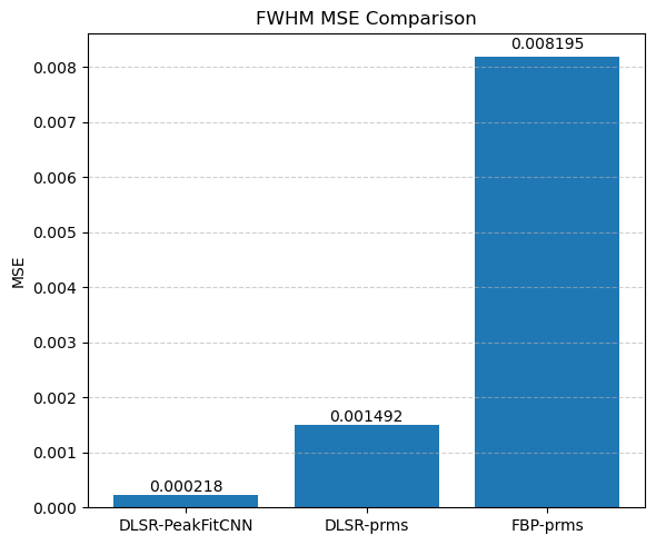
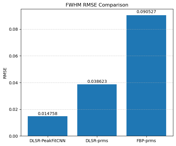
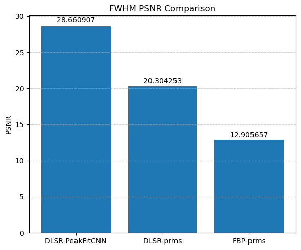
[82]:
gt = peak_slope * msk
cnn = cnn_slope * msk
prms_dlsr = prms_slope_dlsr * msk
prms = prms_slope * msk
print("CNN MAE:", mae(gt, cnn))
print("PRMS DLSR MAE:", mae(gt, prms_dlsr))
print("PRMS MAE:", mae(gt, prms))
print('----------')
print("CNN SSIM:", ssim(gt, cnn))
print("PRMS DLSR SSIM:", ssim(gt, prms_dlsr))
print("PRMS SSIM:", ssim(gt, prms))
print('----------')
print("CNN MSE:", mse(gt, cnn))
print("PRMS DLSR MSE:", mse(gt, prms_dlsr))
print("PRMS MSE:", mse(gt, prms))
print('----------')
print("CNN RMSE:", rmse(gt, cnn))
print("PRMS DLSR RMSE:", rmse(gt, prms_dlsr))
print("PRMS RMSE:", rmse(gt, prms))
print('----------')
print("CNN PSNR:", psnr(gt, cnn))
print("PRMS DLSR PSNR:", psnr(gt, prms_dlsr))
print("PRMS PSNR:", psnr(gt, prms))
plot_results(gt, cnn, prms_dlsr, prms, label='Slope')
CNN MAE: 0.0002011942187838696
PRMS DLSR MAE: 0.0004251532707203293
PRMS MAE: 0.002878232941822127
----------
CNN SSIM: 0.9452899580886321
PRMS DLSR SSIM: 0.5821262562207158
PRMS SSIM: 0.1345862439554213
----------
CNN MSE: 1.199620708520884e-06
PRMS DLSR MSE: 1.7387319958491733e-06
PRMS MSE: 3.512748112242048e-05
----------
CNN RMSE: 0.0010952719792457414
PRMS DLSR RMSE: 0.001318609872497993
PRMS RMSE: 0.005926844111533597
----------
CNN PSNR: 27.168360631586182
PRMS DLSR PSNR: 25.556473713353967
PRMS PSNR: 12.502330082823008
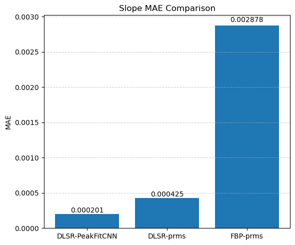
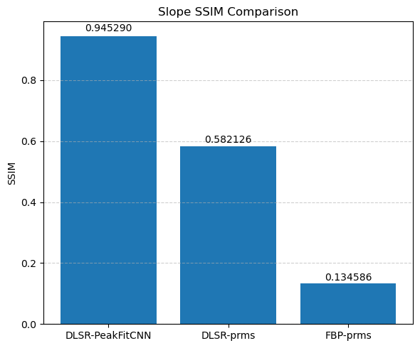
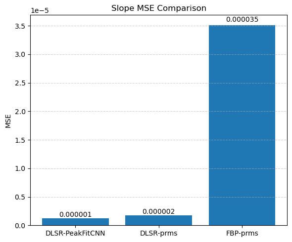
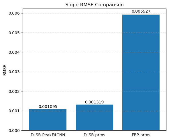
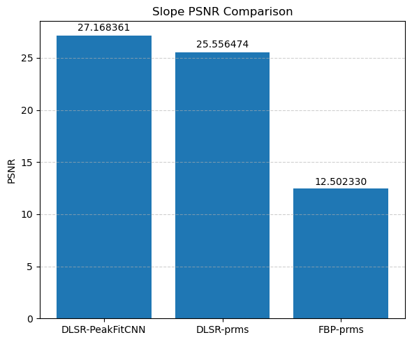
[83]:
gt = peak_intercept * msk
cnn = cnn_intercept * msk
prms_dlsr = prms_intercept_dlsr * msk
prms = prms_intercept * msk
print("CNN MAE:", mae(gt, cnn))
print("PRMS DLSR MAE:", mae(gt, prms_dlsr))
print("PRMS MAE:", mae(gt, prms))
print('----------')
print("CNN SSIM:", ssim(gt, cnn))
print("PRMS DLSR SSIM:", ssim(gt, prms_dlsr))
print("PRMS SSIM:", ssim(gt, prms))
print('----------')
print("CNN MSE:", mse(gt, cnn))
print("PRMS DLSR MSE:", mse(gt, prms_dlsr))
print("PRMS MSE:", mse(gt, prms))
print('----------')
print("CNN RMSE:", rmse(gt, cnn))
print("PRMS DLSR RMSE:", rmse(gt, prms_dlsr))
print("PRMS RMSE:", rmse(gt, prms))
print('----------')
print("CNN PSNR:", psnr(gt, cnn))
print("PRMS DLSR PSNR:", psnr(gt, prms_dlsr))
print("PRMS PSNR:", psnr(gt, prms))
plot_results(gt, cnn, prms_dlsr, prms, label='Intercept')
CNN MAE: 0.005857232838535097
PRMS DLSR MAE: 0.009264647091086672
PRMS MAE: 0.020826641719806915
----------
CNN SSIM: 0.6136655625582432
PRMS DLSR SSIM: 0.4771903437150229
PRMS SSIM: 0.3741221403784698
----------
CNN MSE: 7.792827423047736e-05
PRMS DLSR MSE: 0.00019009746708220906
PRMS MSE: 0.001414121818277489
----------
CNN RMSE: 0.00882769926030998
PRMS DLSR RMSE: 0.013787583801457347
PRMS RMSE: 0.03760481110546214
----------
CNN PSNR: 29.041849587165906
PRMS DLSR PSNR: 25.16903687114867
PRMS PSNR: 16.453931943563802
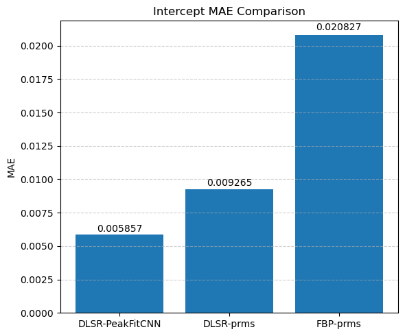

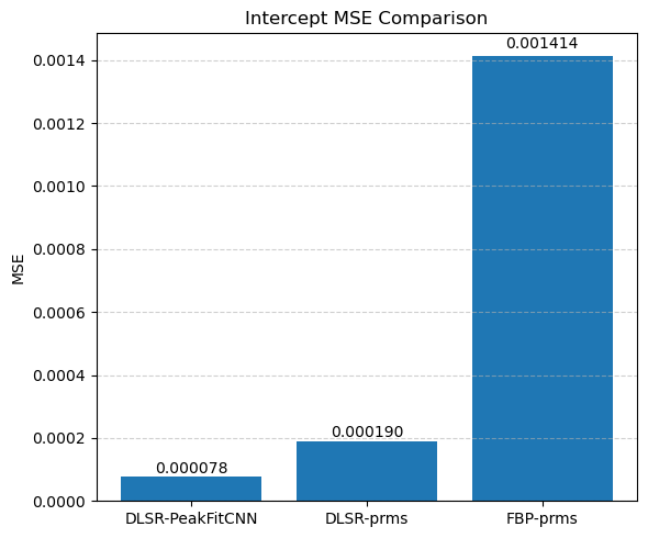

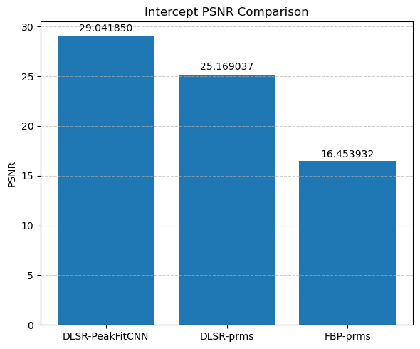
✅ Final Remarks and Outlook
In this notebook, we explored and compared three distinct strategies for reconstructing peak parameter maps from hyperspectral XRD-CT data under angular undersampling conditions:
🧪 Summary of Approaches
Method |
Input |
Output |
Optimization |
|---|---|---|---|
FBP + Peak Fitting |
N/A |
Parameter maps |
Peak fitting using the reconstructed volume |
DLSR-prm |
N/A |
Parameter maps |
Peak fitting and reconstruction of the parameter maps using the sinogram data |
DLSR-PeakFitCNN |
Downsampled hyperspectral volume |
Parameter maps |
Peak fitting and reconstruction of the parameter maps using the sinogram data with a self-supervised neural network |
📊 Key Findings
DLSR-prm provides physically consistent reconstructions and shows some resilience to angular undersampling but the how one imposes constraints and regularisation can change the results significantly.
DLSR-PeakFitCNN performs surprisingly well, achieving smooth and accurate maps with fewer learnable parameters and faster convergence. It benefits from spatial regularization via convolution.
FBP + Peak Fitting shows reasonable accuracy but is sensitive to FBP artefacts, especially near boundaries or in low-signal regions. Its performance degrades more noticeably under sparse sampling.
💡 Contributions
First open-source PyTorch-based implementation of the DLSR framework for XRD-CT
Demonstrated the feasibility of using neural networks instead of parameter maps in DLSR
Introduced self-supervised CNN peak fitting as a lightweight alternative, requiring no ground truth labels
Provided a modular, reproducible benchmarking framework for XRD-CT reconstruction pipelines
🔭 Future Directions
Extend to multi-peak and asymmetric peak shapes (e.g., Pseudo-Voigt or split-Voigt)
Apply to real experimental datasets, especially where parallax or low-angle artefacts dominate
Combine DLSR and CNN strategies in hybrid architectures, e.g., CNN-based priors in physics-constrained models
This work lays the groundwork for robust, interpretable, and scalable peak fitting in next-generation XRD-CT datasets. The integration of physics-based modeling and deep learning opens exciting opportunities for real-time, high-fidelity chemical imaging.